Nbody6tid Manual
Andreas Ernst
Astronomisches Rechen-Institut am
Zentrum für Astronomie der Universität Heidelberg,
Mönchhofstr. 12-14, 69121 Heidelberg, Germany
Version 06/2012
Nbody6tid Manual
Andreas Ernst
Astronomisches Rechen-Institut am
Zentrum für Astronomie der Universität Heidelberg,
Mönchhofstr. 12-14, 69121 Heidelberg, Germany
Version 06/2012
This manual is intended to be a documentation for students and postdocs of the three variants NBODY6TID, NBODY6TIDPAR and NBODY6TIDGPU of Sverre Aarseth’s direct N-body code NBODY6. The author would like to note that that the name NBODY6TID and the first simple version of this program stem from Rainer Spurzem. For a documentation of NBODY6 the reader is first and foremost referred to the webpage of Sverre Aarseth (http://www.ast.cam.ac.uk/~sverre/) which contains a code repository as well as documentation and to the manual NBODY6++ - Features of the computer-code by Emil Khalisi and Rainer Spurzem. Only if the reader is interested to solve the N-body problem in the tidal field of a galaxy such as the Milky Way (which can be represented as a 3-component Plummer-Kuzmin model with special parameters), that of a galactic center (with a power-law gravitational potential) or in other special tidal fields like that of a Plummer or Dehnen model, this manual may be useful to him.
Heidelberg, June 2012
Andreas Ernst
The programs NBODY6TID, NBODY6TIDPAR and NBODY6TIDGPU are three variants of the direct N-body code NBODY6 by Sverre Aarseth (Aarseth 1999, 2003). They integrate the N-body problem in an analytic background potential of a galaxy or a galactic centre.
The special feature of NBODY6TID, NBODY6TIDPAR and NBODY6TIDGPU is the implementation of different tidal fields. This implementation is based on the implementation in the (parallel) code NBODY6GC which is described in detail in Ernst, Just & Spurzem (2009) and Ernst (2009). Several analytic models for the background potential are now implemented, e.g.,
In addition to the equations of motion of the N-body problem, NBODY6TID solves the equations of motion of the star cluster orbit around the Galactic center with an eighth-order composition scheme (Yoshida 1990; for the coefficients see McLachlan 1995). The tidal force of the background potential acts on all particles in the N-body system and is added as a perturbation to the KS regularization (Kustaanheimo & Stiefel 1965) of NBODY6.
NBODY6TID is able to integrate star cluster orbits with almost all eccentricities. For nearly radial orbits a time transformation can be switched on to guarantee an exact orbit integration during the pericenter passages. The leapfrog-like symplectic integration schemes allow for adaptive time steps if one applies a Sundman transformation to the time (Sundman 1912, Mikkola & Tanikawa 1999, Preto & Tremaine 1999, Mikkola & Aarseth 2002).
It is also possible to switch on a semianalytical treatment of Chandrasekhar’s dynamical friction with different χ functions and different realizations of the Coulomb logarithm, i.e. fixed or variable according to Just & Peñarrubia (2005). Since the symplectic composition schemes are by construction suited to Hamiltonian systems, the dissipative dynamical friction force requires special attention. It is implemented in NBODY6TID with an implicit midpoint method using an iteration (see, e.g., Mikkola & Aarseth 2002).
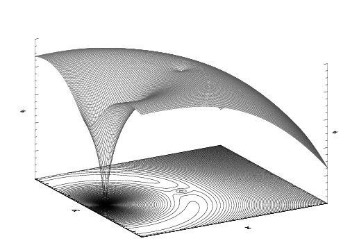
The tidal field (or effective tidal potential) is given by the superposition of the galactic gravitational potential and the centrifugal potential, i.e. we usually have
![1 [ ]
Φeff,tid(x,y,z) = Φ (x + RC,y,z)-- Ω2 (x+ RC )2 + y2 .
2](nb6tidmanual0x.png) | (1) |
where RC is the radius of the circular orbit. For a circular orbit, the tidal field resembles a ring-like parabolic (to second order) ridge around the galactic center (see figure on the title page). In this ridge the star cluster potential is embedded. For a spherically symmetric star cluster potential the equilibrium Lagrange points L1 - L5 naturally arise. Therefore the total gravitational potential is given by
 | (2) |
Here the origin is shifted to the star cluster center at (x,y,z) = (0,0,0). For the star cluster potential, a Plummer model can be inserted.
We define r =  for the spherically symmetric models, where x,y andd z are
Cartesian coordinates. G is the gravitational constant and M a mass. The velocity components are
vx,vy and vz.
for the spherically symmetric models, where x,y andd z are
Cartesian coordinates. G is the gravitational constant and M a mass. The velocity components are
vx,vy and vz.
The Kepler potential is given by
 | (3) |
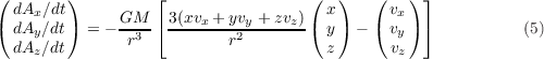
The acceleration is given by
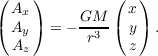 | (4) |
The jerk is given by
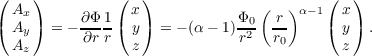
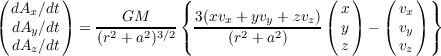
The spherically symmetric power-law or scale-free models have a potential of the form

where r is the radius and r0 is a length unit. The acceleration has the form
 | (7) |
The jerk is given by
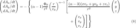
A supermassive black hole can be added to the center of such a model.
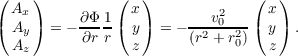
The gravitational potential of a Plummer model (Plummer 1911) is given by
 | (9) |
where a is the Plummer radius. The acceleration is then given by
 | (10) |
The jerk is given by
 | (11) |
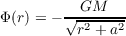
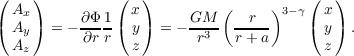
The gravitational potential of a Dehnen model (Dehnen 1993, Tremaine et al. 1994) is given by
![[ ( ) ]
GM----1-- --r-- 2-γ
Φ (r) = - a 2 - γ 1 - r+ a](nb6tidmanual12x.png) | (12) |
where a is a scale radius. The acceleration is then given by
 | (13) |
The jerk is given by
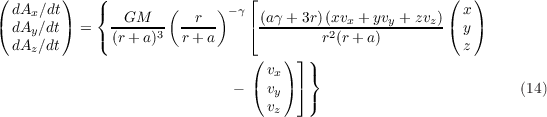
A logarithmic gravitational potential is given by
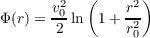 | (15) |
The acceleration is given by
 | (16) |
The jerk is given by
 | (17) |
| Component | M [M⊙] | a [kpc] | b [kpc] |
| Bulge | 1.4 × 10¹⁰ | 0.0 | 0.3 |
| Disk | 9.0 × 10¹⁰ | 3.3 | 0.3 |
| Halo | 7.0 × 10¹¹ | 0.0 | 25.0 |
| Rg [kpc] | V cir [km s-1] | Rg [kpc] | V cir [km s-1] |
| 0.5 | 279.269858420500 | 10.5 | 231.472619038406 |
| 1.0 | 246.015548276821 | 11.0 | 231.416801583084 |
| 1.5 | 230.132164798490 | 11.5 | 231.499317939399 |
| 2.0 | 228.141259503200 | 12.0 | 231.704811326295 |
| 2.5 | 231.286020479153 | 12.5 | 232.017589382089 |
| 3.0 | 235.208140475138 | 13.0 | 232.422164626838 |
| 3.5 | 238.261145511816 | 13.5 | 232.903626883944 |
| 4.0 | 240.070687448505 | 14.0 | 233.447890039686 |
| 4.5 | 240.763498292986 | 14.5 | 234.041845222914 |
| 5.0 | 240.613878677284 | 15.0 | 234.673444774045 |
| 5.5 | 239.899715058196 | 15.5 | 235.331735556181 |
| 6.0 | 238.853489734555 | 16.0 | 236.006855744588 |
| 6.5 | 237.652904859520 | 16.5 | 236.690005856049 |
| 7.0 | 236.426154512127 | 17.0 | 237.373402187912 |
| 7.5 | 235.261261678691 | 17.5 | 238.050218839306 |
| 8.0 | 234.215362687272 | 18.0 | 238.714522944716 |
| 8.5 | 233.322594742001 | 18.5 | 239.361206558702 |
| 9.0 | 232.600357491854 | 19.0 | 239.985917711179 |
| 9.5 | 232.054117466732 | 19.5 | 240.584992445018 |
| 10.0 | 231.681026811365 | 20.0 | 241.155389105121 |
| Rg [kpc] | β | Rg [kpc] | β |
| 0.5 | 1.3605 | 10.5 | 1.4059 |
| 1.0 | 1.2520 | 11.0 | 1.4153 |
| 1.5 | 1.3474 | 11.5 | 1.4245 |
| 2.0 | 1.4342 | 12.0 | 1.4333 |
| 2.5 | 1.4737 | 12.5 | 1.4415 |
| 3.0 | 1.4781 | 13.0 | 1.4490 |
| 3.5 | 1.4639 | 13.5 | 1.4558 |
| 4.0 | 1.4425 | 14.0 | 1.4619 |
| 4.5 | 1.4201 | 14.5 | 1.4671 |
| 5.0 | 1.4002 | 15.0 | 1.4715 |
| 5.5 | 1.3843 | 15.5 | 1.4751 |
| 6.0 | 1.3728 | 16.0 | 1.4780 |
| 6.5 | 1.3658 | 16.5 | 1.4802 |
| 7.0 | 1.3627 | 17.0 | 1.4816 |
| 7.5 | 1.3631 | 17.5 | 1.4824 |
| 8.0 | 1.3664 | 18.0 | 1.4825 |
| 8.5 | 1.3719 | 18.5 | 1.4821 |
| 9.0 | 1.3791 | 19.0 | 1.4812 |
| 9.5 | 1.3874 | 19.5 | 1.4798 |
| 10.0 | 1.3965 | 20.0 | 1.4779 |
The parameters of the 3-component Plummer-Kuzmin model (Miyamoto & Nagai 1975) of the Milky Way are given in table 1 or Just et al. (2009). The total gravitational potential is given by a a superposition of three potentials for bulge, disk and halo. A few quantities as a function of galactocentric radius are given in tables 2 and 3. The gravitational potential has the form
 | (18) |
The acceleration for the Plummer-Kuzmin model is given by the expression
![( ) ( ) ( x )
( Ax) ( dΦ ∕dx) ------------ GM----------- ( y )
Ay = - dΦ ∕dy = [ 2 2 √-2---2 2]3∕2 ⋅ a+√b2+z2
Az dΦ ∕dz x +y + (a + b + z ) z ⋅ √b2+z2](nb6tidmanual19x.png) | (19) |
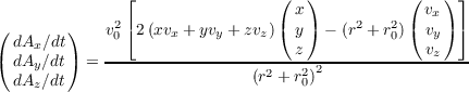
The jerk is given by the lengthy expressions
![{ [ ( )] [ ( √ ------)2]}
dAx GM 3x xvx + yvy + zvz √b2a+z2 + 1 - vx x2 + y2 + a+ b2 + z2
dt--= -------------------[--------(---√-------)2]5∕2-------------------
x2 + y2 + a+ b2 + z2](nb6tidmanual20x.png) |
![{ [ ( )] [ ( √ ------)]}
dA GM 3y xvx + yvy + zvz √b2a+z2 + 1 - vy x2 + y2 + a+ b2 + z2 2
--y-= -------------------[--------(---√-------)2]5∕2-------------------
dt x2 + y2 + a+ b2 + z2](nb6tidmanual21x.png) |
![{ √ -2---2[ ( ) ]
dAz-= GM 3za+√---b-+-z- xvx +yvy + zvz √---a---+ 1
dt b2 + z2 b2 + z2
[ ( ∘ ------)2] [(a + √b2 +-z2) ] }
- vz x2 + y2 + a+ b2 + z2 × ---√--------- - z2----a--3∕2- /
b2 + z2 (b2 + z2)
[ ( ∘ ------)2]5∕2
x2 + y2 + a+ b2 + z2 (20)](nb6tidmanual22x.png)
which also depend on the velocity components.
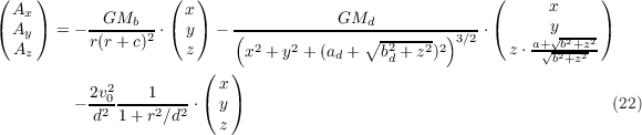
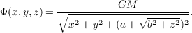
The gravitational potential of the JSH95 model (see Dinescu et al. 1999) is given by
 | (21) |
with Mb = 3.4 × 10¹⁰M⊙, c = 0.7 kpc, Md = 1011M⊙, ad = 6.5 kpc, bd = 0.26 kpc, v0 = 128 km s-1, d = 12.0 kpc. The bulge has a Hernquist profile, the disk is represented as a Plummer-Kuzmin model and the halo by a logarithmic potential.
The acceleration for the JSH95 model is given by the expression
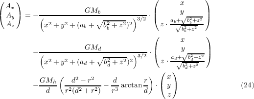
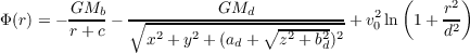
The gravitational potential of the P90 model (see Dinescu et al. 1999) is given by
![Φ (r) = - ∘--------GMb------------- ∘---------GMd------------
x2 + y2 + (a + ∘z2-+-b2)2 x2 + y2 + (a + ∘z2-+-b2)2
[ ( b ) b ] d d
+ GMh-- 1ln 1 + r2 - d arctan r (23)
d 2 d2 r d](nb6tidmanual25x.png)
with Mb = 1.12 × 10¹⁰M⊙, ab = 0.0 kpc, bb = 0.277 kpc, Md = 8.0710M⊙, ad = 3.7 kpc, bd = 0.20 kpc, Mh = 5 × 10¹⁰M⊙, d = 6.0 kpc.
The acceleration for the P90 model is given by the expression
All new subroutines in NBODY6TID begin with the letters “EXT” for “EXTernal tidal field” or “EXTernal galaxy”. Table 4 gives an overview of the routines with a short description.
| Subroutine | Description | Called by subroutine |
| EXTINIT | GC initializations | START |
| EXTGALAX | GC external force on star cluster | REGINT, KSPERT |
| EXTGALAX2 | Calculates all galaxy quantities | OUTPUT, EXTINIT, EXTINT, |
| EXTCHECK, EXTMASS, EXTCHI, | ||
| EXTXCOUL | ||
| EXTFORCE | Calculate GC force | EXTINT, EXTGALAX |
| EXTFPR | Time transformation (optional) | EXTINIT, EXTINT |
| EXTINT | GC integrator | INTGRT |
| EXTCHECK | GC energy check | ADJUST, OUTPUT |
| EXTENERGY | Calculate GC energy | EXTCHECK, EXTINIT, EXTINT, |
| EXTMASS | ||
| EXTMASS | Star cluster mass and members | EXTINIT, EXTINT |
| EXTOUTP | GC data output | OUTPUT |
| EXTIPOL | Interpolation of GC jerk if not known | EXTINT |
| EXTCHI | Calculates current value of χ | EXTINT, EXTOUTP |
| EXTXCOUL | Calculates current value of lnΛ | EXTINIT, EXTOUTP |
The following changes have been made to the original program NBODY6:
Shown below are two examples of the additional input file called galax.dat which contains the parameters of the external tidal field.
The input variables have the following purpose:
For the planning of a new run or even a parameter space you should invest some time. To setup a run, you need to choose the parameter of the star cluster and the galaxy in which the star cluster is orbiting, the parameters of the orbit (i.e., the eccentricity and positioning of the orbit, should dynamical friction be turned on?). Then you must change the input files in and galax.dat accordingly. It is always useful to calculate also the relevant time scales. Let us define that rV and tV are the N-body units of length and time. We have rV = RBAR pc. Then the setup of a run proceeds as follows:
 Myr
Myr
 tV
tV
If you want to use the code, you need to compile it first. The current standard Fortran 77 compiler is gfortran, but you may use ifort or pgf77 as well. However, you must change the Makefile, Makefile_gpu and Makefile_sse appropriately. For the GPU version you need a machine which is equipped with a GPU. For the parallel version you need access to a parallel cluster or a supercomputer. The main routines of the standard serial code are in the folder /Ncode, the GPU routines are in the folder /GPU and its subfolder /GPU/lib. The stand-alone version of the parallel code is located in the folder /PAR. In the subfolders /GPU/run and /PAR/run are examples of the input files in, inmod (the restart input file) and galax.dat for the 3-component Plummer-Kuzmin (3PLK) model and the scale-free (SCF) model. Important: The variable KZ(14) must be set to the value KZ(14)=5 in the standard input file of NBODY6.
The following commands depend on the specific architecture of the parallel cluster or supercomputer. When you are submitting a job to a small Beowulf cluster, you typically have to use a queue submission command like qsub within a console. When you are submitting to a large supercomputer, you may have to make use of a submission client like UNICORE with a comfortable graphical user interface. For GRID jobs you may also have to use the console-based GLOBUS toolkit.
In the run folder there are backup scripts called backup.sh and restore.sh. They can be used if a run has stopped for some reason and will be restarted several times. The backup script tests whether a backup already exists. Usage:
The important output files of nbody6 are backed up under a number and can be restored.
There is also a script called clean.sh which cleans up the run directory:
The programs “snap.f” (and “snaprho.f”) calculate a snapshot at a certain time in the format
For the calculation of the density the procedure described in Casertano & Hut (1985) is applied. The number of neighbors (e.g. Nnb = 5 - 20) is a free parameter.
The additional data output of NBODY6TID has the following form. You may type something like
to obtain a file with the coordinates of the galactic center.
The folder “/IntExt” contains a simple integrator called INTEXT (“INTegrate EXTernal galaxy”) for star cluster orbits in the tidal field.1 The only difference to NBODY6TID is that the N-body problem is not solved. Therefore the integration is very fast.
Usage: Adapt galax.dat input file to your needs.2 Then start the program as follows:
At the end of the integration the relative energy error is printed out. Make sure that it is sufficiently small.
Thanks go to Dr. Sverre Aarseth, Prof. Dr. Rainer Spurzem, Dr. Keigo Nitadori, Dr. Peter Berczik, Dr. Andreas Just, Prof. Dr. Ortwin Gerhard, Dr. Kap Soo Oh and Dr. Godehard Sutmann. Further thanks go to those who contributed to NBODY6TID through discussions, mainly the members of the stellar dynamics group at ARI.
[1] Aarseth S. J., 1999, PASP, 111, 1333
[2] Aarseth S. J., 2003, Gravitational N-body simulations - Tools and Algorithms, Cambridge Univ. Press, Cambridge, UK
[3] Binney J., Tremaine S., Galactic Dynamics, 2008, 2nd ed., Princeton Univ. Press, Princeton, USA
[4] Casertano S., Hut P., 1985, Ap. J., 298, 80
[5] Dehnen W., 1993, MNRAS, 265, 250
[6] Dinescu D.I., Girard T. M., van Altena W. F., 1999, AJ, 117, 1792
[7] Ernst A., 2009, Dissolution of star clusters in the Galaxy and its Center, PhD thesis, Univ. of Heidelberg, Germany, http://www.ub.uni-heidelberg.de/archiv/9375
[8] Ernst A., Just A., Spurzem R., 2009, MNRAS 399, 141
[9] Gürkan M. A., Freitag M., Rasio F. A., 2004, Ap. J., 604, 632
[10] Just A., Peñarrubia J., 2005, A&A, 431, 861
[11] Just A., Berczik P., Petrov M.I., Ernst A., 2009, MNRAS, 392, 969
[12] Kustaanheimo P. Stiefel E. L., 1965, J. für reine angewandte Mathematik, 218, 204
[13] McLachlan R., 1995, SIAM J. Sci. Comp., 16, 151
[14] Mikkola S., Tanikawa K., 1999, Cel. Mech. Dyn. Astron., 74, 287
[15] Mikkola S., Aarseth S. J., 2002, Cel. Mech. Dyn. Astron., 84, 343
[16] Miyamoto M., Nagai R., 1975, PASJ 27, 533
[17] Nitadori K., Aarseth S. J., 2011, MNRAS, submitted
[18] Plummer H. C. 1911, MNRAS 71, 460
[19] Preto M., Tremaine S. 1999, AJ, 118, 2532
[20] Spurzem R., 1999, J. Comp. Appl. Maths, 109, 407
[21] Sundman K. F., 1912, Acta Math., 36, 105
[22] Tremaine S. et al., 1994, AJ, 107, 634
[23] Yoshida H., 1990, Phys. Lett. A, 150, 262