Andreas Ernst
The few-body problem and other selected topics in
computational physics
.
.
.
Es ist der Weisheit fromme Ehre,
. Inhaltsverzeichnis
Foreword
1 The few-body problem 1.1 Introduction to the two-body problem 1.2 Initial conditions for three- and four-body problems 1.3 Few-body units 1.4 Taylor integrators 1.5 Leapfrog/Verlet integrators 1.5.1 Standard Leapfrog methods 1.5.2 Logarithmic Hamiltonian method (LogH) 1.5.3 Time-transformed leapfrog (TTL) 1.5.4 Higher-oder composition schemes 1.6 Hermite integrators 1.6.1 Standard Hermite method 1.6.2 Iterated time-symmetric Hermite method 1.6.3 Higher-order Hermite methods 1.6.4 Adaptive time steps for the Hermite scheme 1.7 Runge-Kutta integrators (RK) 1.8 Tasks 2 Galactic dynamics 2.1 Spherically symmetric models 2.1.1 Mechanical foundations 2.1.2 Kepler potential 2.1.3 Power-law models 2.1.4 Plummer model 2.1.5 Dehnen models 2.1.6 Logarithmic potential 2.2 Multi component models 2.2.1 The 3PLK Milky Way model 2.2.2 JSH95 Milky Way model 2.2.3 P90 Milky Way model 2.2.4 Zotos’ barred spiral galaxy model 2.3 Tasks 3 Linear stability analysis 3.1 Introduction to linear stability analysis 3.2 Logistic Map (1D) 3.3 Hénon-Heiles system (2D) 3.4 Lotka-Volterra system (2D) 3.5 Lorenz attractor (3D) 3.6 Rössler attractor (3D) 3.7 Tasks 4 Integrating the stellar initial mass function 4.1 Integral solving 4.1.1 Solving a differential equation 4.1.2 Using geometrical rules 4.1.3 Monte-Carlo integration 4.2 Tasks 5 Astrophysical Poisson equations 5.1 Lane-Emden equation 5.1.1 Chandrasekhar mass 5.1.2 Isothermal case 5.2 Tasks Afterword References A Solutions and hints for some exercises B TTL program C Gnuplot examples D Three-body animations Foreword The integration of differential equations and the numerical solution of integrals has gained much attention since the flowering of computer technology in the natural sciences. This book, which is called “Simply Integrate!’, contains descriptions of a collection of different integrators such as Taylor methods, Leapfrog methods, Hermite schemes, 2nd, 4th and 8th-order Runge-Kutta methods, or fancy ones, like a time-transformed 8th-order composition scheme where the highest accuracy is needed. An example are highly unstable periodic solutions of the three-body problem. In extreme cases one uses a “shooting method” from both sides to obtain closed orbits. A measure for the degree of instability is the dominant eigenvalue of the monodromy matrix in Floquet theory, which is not covered in this book, but for example in the book by Contopoulos (2002). The biggest part of the present book is concerned with “science that is hoary with age” (Platon, Timaios) but parts of it are also concerned with novel inventions and methods of modern physics and astrophysics. The first main chapter of the present book is dedicated to the few-body problem. Starting with an introduction to the two-body problem, which is analytically solvable the author presents initial conditions for three- and four-body problems. These can be solved with the hereafter presented integration methods mentioned above. If heuristically means “concerning the inventions”, one may say: The chapter proceed heuristically, from simple to complex algorithms, from the two-body problem to the few-body problem. The second main chapter of this book is about galactic dynamics and orbital mechanics in analytic gravitational potentials. At first spherically symmetric models of stellar systems are discussed and later multi compenent models of galaxies. The aim is to integrate orbits in these potentials with a self-written integrator, against the “ignava ratio”. The third main chapter of this book is dedicated to linear stability analysis. The linear stability analysis is presented with many examples. Every example uses a general classification of equilibrium points, which is presented in the beginning. In this sense, the individual case is explained by summing it under a general classification or mathematical law. This is the paradigmatic method of the nomothetical sciences (Hempel, 1977; Gadamer, 1990). Further chapters are concerned with the stellar initial mass function and astrophysical Poisson equations. The field of work of the author of this book is “experimental stellar dynamics”. The word “experimental” means in the context of astrophysics, that computer experiments are being used to study the dynamical evolution of stellar systems, where stars interact through gravity. Since the author’s N-body simulations require a huge amount of computer power, he has made use of Beowulf PC clusters as well as the largest supercomputers in Europe, field programmable gate arrays (FPGAs), graphics processing units (GPUs) and the grid technology. For the plots in this book, GNUPLOT, IDL, R, OMNIGRAFFLE and GIMP have been used. A website of this book with more material can be found at the internet address http://www.simplyintegrate.de. On the one hand, the readers of this book should get an impression what it means to do computational physics, on the other hand, they should see how much fun it is! And the scientist and truth seeker, who has once read the book Burning Daylight by Jack London, knows well about the comparableness between the scientific research and the utterly exhausting search for gold nuggets at the Klondike River. It remains, to exclaim from time to time with Jack London’s hero: “Burning daylight!”
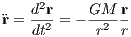
Heidelberg, im Mai 2014 1 The few-body problem1.1 Introduction to the two-body problemWe follow the lecture notes of Kühn & Spurzem (2005) first. A similar approach to the problem can be found in the book by Binney & Tremaine (2008). Newton’s equation of motion for the relative motion of two bodies under their mutual gravitational force is
where G is the gravitational constant, M = m1 + m2 is the total mass, r = (x2 - x1,y2 - y1,z2 - z1) the
relative vector, r = |r| the relative distance and the two dots denote a second derivative with respect to time t
in the notation of Newton. The bound solutions of Eqn. (1.1) are ellipses, the general solutions are conic
sections. Kühn & Spurzem (2005) note that the Hamiltonian of the relative motion leads to
μ Numerical solution: For a numerical integration we need to replace Eqn. (1.1) by two coupled first-order differential equations,
Note that these cannot be solved independently. A dimensionless formulation can be introduced (e. g. Kühn & Spurzem, 2005). We define
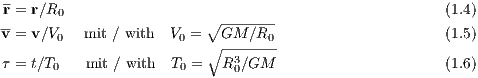 Using this we obtain
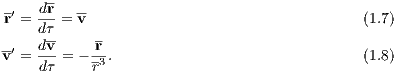
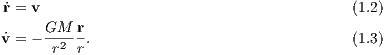
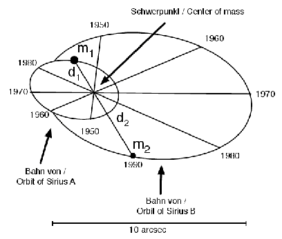
Abbildung 1: Left: Measuring the sum of masses M = m1 + m2 from the relative motion. Right:
Measuring the mass ratio m1∕m2 = d2∕d1 from the motion of the double star components around their
common center of mass. According to Green & Jones (2003). Graphics program: OMNIGRAFFLE.
where the prime denotes a derivative with respect to the scaled time τ in the notation of Lagrange. The simplest Taylor integrator, the Euler integrator, can be written as Euler-Methode / Euler method:  where a = v′ = dv∕dτ is the dimensionless acceleration, Δt is the time step and the subscripts ‘0’ (and ‘1’)
stand for the current (next) time step. The local error (in one time step) of the Euler method is of order
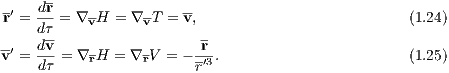
a0(Δt)2 in position and Although it is possible to implement the Euler scheme straightforwardly in the form of a computer program, the author recommends to begin the integration exercises with the initial conditions for three- and four-body problems given in the next section. The reason is that the computer program should be written generally enough, such that a few-body problem with N > 2 can be solved, where the variable N stands for the particle number. Integrals of motion: We prove the temporal constancy of the integrals of the relative motion,
 where r = |r| and v = |v|. We use the Graßmann identity
We use Eqn. (1.14) to calculate
and find
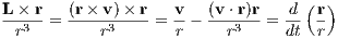
 Analytical solution: For an analytical solution of Eqn. (1.1) we consider the expression
This can be written as
![ercos(ψ - ψ )+ r = -L2- oder ∕ or (1.20)
[ 0 ] GM
---L2∕(GM-)----
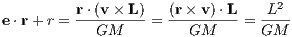
r = 1+ ecos(ψ- ψ0), (1.21)](simplyhtml18x.png) which is the well-known solution of a conic section with the orbital plane (e. g. Kühn & Spurzem, 2005) with the phase angle ψ = ψ(t). Hamiltonian formulation: The conserved Hamiltonian is given by
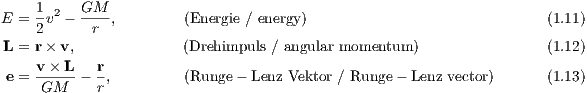
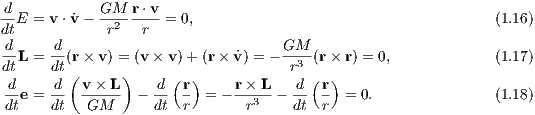
where T and V are kinetic and potential energy, respectively, and H0 a constant. With the dimensionless expressions for the relative motion of the two-body problem
we obtain
 where we have used the separability property of the Hamiltonian, according to which T = T(v)
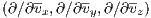
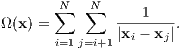
depends only on v and V = V (r) depends only on r. The notations of the gradient operators
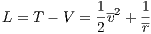
are ∇r ⋅ = Lagrangian formulation: The Lagrange function is given by
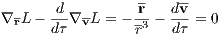
in dimensionless phase space coordinates. The Euler-Lagrange equations of motion are given by
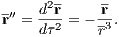
or
We recognize the dimensionless formulation of Eqn. (1.1). 1.2 Initial conditions for three- and four-body problemsThe initial conditions are given in the form m x y z vx vy vz. Acht / Eight
1 0.9700436 -0.24308753 0 0.466203685 0.43236573 0
1 -0.9700436 0.24308753 -0 0.466203685 0.43236573 0 1 0 0 0 -0.93240737 -0.86473146 -0
Pytagoreisches Problem / Pythagorean problem
3 1 3 0 0 0 0
4 -2 -1 0 0 0 0 5 1 -1 0 0 0 0
Herz / Heart
1 -5.54504183347047 0 0 0 -0.414526370749686 0
1 2.772520916735235 -1.678453738023547 0 0.3933483781289587 0.207263185374843 0 1 2.772520916735235 1.678453738023547 0 -0.3933483781289587 0.207263185374843 0
Schwimmer / Swimmer
1 0 0 0 0 1.2050 0
1 -1 0 0 0 -0.6025 0 1 1 0 0 0 -0.6025 0
Ducati / Ducati
1 -1 0 0 0 -0.93932504689 0
1 0.5 -0.647584 0 -0.505328085163 0.46962523449 0 1 0.5 0.6475840 0 0.505328085163 0.46962523449 0
Stern / Star
1 1.0598738926379 1.7699901770118 0 -0.55391384867197 -0.39895079845794 0
1 0 -0.80951135793043 0 1.0936551555351 0 0 1 -1.0598738926379 1.7699901770118 0 -0.55391558212647 0.39895379682134 0 1 0 -2.7304689960932 0 0.01417427526245 0 0
Special solutions of the three- or four-body problem are described in: Szebehely & Peters (1976); Hénon (1976); Moore (1993); Simó (2000); Chencincer & Montgomery (2000); Broucke (2002); Vanderbei (2004); Martynova & Orlov (2009); Šuvakov & Dmitrašinović (2013); Ouyang & Xie (2013).
After a discussion of the unit scaling in the next section many different integration algorithms are described in following sections. The author recommends, after writing your own integration program according to one of these algorithms, to begin the integration exercises with the figure “eight”, since it is easy to integrate due to its stability and the fact, that close encounters do not occur at all. Afterwards, you may try to solve the Pythagorean problem. The Pythagorean problem is difficult to integrate. A very accurate integrator must be used which is able to cope with the numerous close encounters. In addition to the initial conditions for the figure “heart” mentioned above we also state the initial conditions for two other choreographic solutions (Simó, 2000): Choreographie 1 / choreography 1
0.3333333333333333 -0.39636722 0 0 0 -0.809132789 0
0.3333333333333333 0.19818361 -0.12376832 0 0.673306125 0.404566394 0 0.3333333333333333 0.19818361 0.12376832 0 -0.673306125 0.404566394 0
Choreographie 2 / choreography 2
0.3333333333333333 -1.56895624 0 0 0 -0.195438179 0
0.3333333333333333 0.784478120 -0.10133157 0 0.631767478 0.097719082 0 0.3333333333333333 0.784478120 0.10133157 0 -0.631767478 0.097719082 0
Particularly the second solution is highly unstable. A “shooting method” from both sides in combination with a highly accurate integrator is recommended to obtain a closed solution. For this purpose, the sign of the velocity vectors must be reversed. Then one integrates (“shoots”) from both sides, once with the standard initial conditions and once with the initial conditions with reversed signs of the velocity vectors. If the accuracy is high enough, one may hope that the solutions meet each other in the middle after half an orbital period. For further choreographies of the three-body problem we refer to the works of Carles Simó. 1.3 Few-body unitsWe follow the procedure from Sverre Aarseth’s direct N-body program NBODY6 (Aarseth, 1999, 2003), but extend the method for the purpose of scaling to arbitrary units. We assume that the N-body system has units in which the gravitational constant has the value G the total mass has the value M and the total energy has the value E. We would like to scale to units in which these quantities have the values G′, M′ and E′. For example, we might be interested in scaling to standard N-body units according to Heggie & Mathieu (1986), which are defined by G′ = M′ = -4E′ = 1. Or, for example, we might want to scale a double or triple star system to physical units, in which G′ = (222.3)-1 pc3M⊙-1Myr-2, M′ = 1 M⊙ and E′ = 1 M⊙pc2Myr-2. We must proceed as follows: Calculation of the total mass: We calculate the total mass firstly,
where N is the number of particles. Translation into the center of mass system: We calculate the center of mass and its velocity,
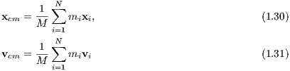 If necessary (xcm ⁄= 0 or vcm ⁄= 0), we apply a translation to the center of mass frame,
 where the prime denotes the quantities in the center of mass frame.
Calculation of the energy: Now we calculate the total energy in the center of mass frame,
where T and V are kinetic and potential energy. It can be seen that the positions and velocities are coupled through the masses, which enter quadratically in the potential energy, and the coupling constant G. Scaling the masses, positions and velocities: We define three scaling factors
We may set
for standard N-body units (Heggie & Mathieu, 1986). Then we scale the individual masses, positions and velocities as follows:
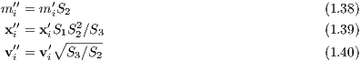 That’s it. The system has now units in which the gravitational constant has the value G′, the total energy is E′ and the total mass is M′. 1.4 Taylor integrators
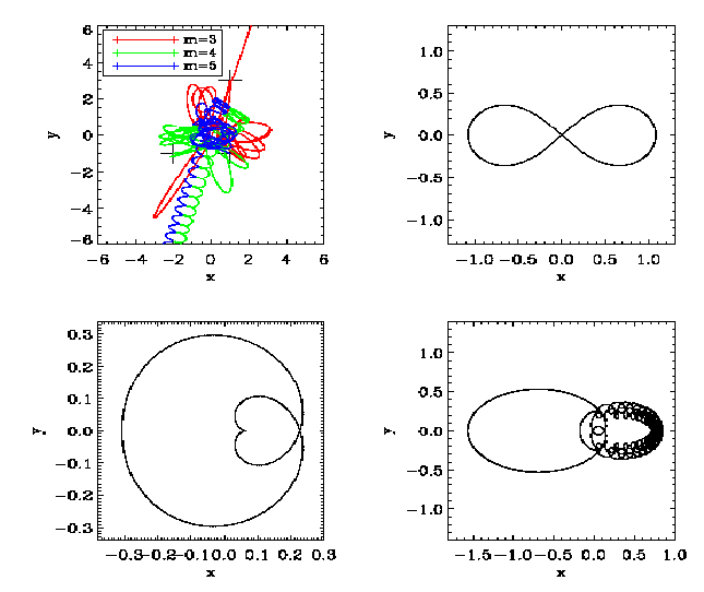
Abbildung 2: Top left: Numerical solution of Burrau’s problem (“The Pythagorean Three-Body
Problem”). Top right: The figure “eight” solution. Bottom left: The “heart”. Bottom right: Strongly
unstable choreographic solution. A “shooting method” from both sides was used to obtain closed orbits.
Plotting language: IDL.
Taylor integrators are based on the evaluation of the Taylor series
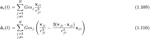
 with Δt = (t-t0), where x1,v1, x0 and v1 are the positions and velocities at the next and current time. The simplest Taylor integrator is the Euler integrator which is first-order accurate. The acceleration and its time derivatives for the Newtonian gravitational force are given by
where xij = xj - xi and xij = |xij| are the relative position of particles j and i and its modulus. Note that for ai(2) and ai(3) more than one summation have to be carried out which is numerically expensive.
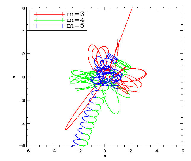
Abbildung 3: Enlargement of the numerical solution of Burrau’s problem (“The Pythagorean
Three-Body Problem”) from Figure 2. Historical facts about Burrau’s problem can be found in
Burrau (1913), Szebehely & Peters (1976) and Peetre (1997). Plotting language: IDL.
1.5 Leapfrog/Verlet integrators1.5.1 Standard Leapfrog methodsHamiltonian flow: As a first “tool” we will introduce the Hamitonian flow. The Poisson brackets are given by
where X = X(x,v,t) and Y = Y (x,v,t) are two “observables”, i.e. differentiable functions of the phase space coordinates x,v and time t (e. g. Kuypers, 1997). We define operators with a hat as
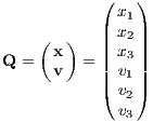
where ⋅ denotes a placeholder. Furthermore, we define the 6-component phase space vector as
We note that
The above equations (1.50) are called “flow equations” for the phase space coordinate Qi. They are equivalent to the Hamiltonian equations of motion, which are written in standard notation as
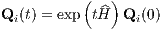
The solution of the flow equations (1.50) can be written formally as
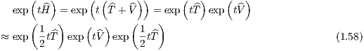
where exp Baker-Campbell-Hausdorff identity: As a second “tool”, we introduce the Baker-Campbell-Hausdorff (BCH) identity: The product of the exponentials of any non-commutative operators X and Y can be expanded as
with
to second order. It we apply the BCH identity twice we can find
with
which is also second-order accurate. Leapfrog schemes: The Leapfrog methods are based on the splitting of the Hamiltonian,
where the kinetic energy T = T(v) depends only on the velocities and the potential energy V = V (x) depends only on positions. Let us call this property the “separability property”. We can write
 where the last approximate equality is valid because of the expansion (1.56). The Hamiltonian equations of motion (1.50) can be written second-order accurate as
or alternatively as
Switching to the standard notation we can obtain from (1.60)
Therefore the integration can be performed in three time-ordered steps. Here we need to consider the
time-ordering of the operators with a hat which is dictated by the fact that they are non-commutative. Note
that the time ordering can also be written formally by applying the Wick-Dyson time ordering operator
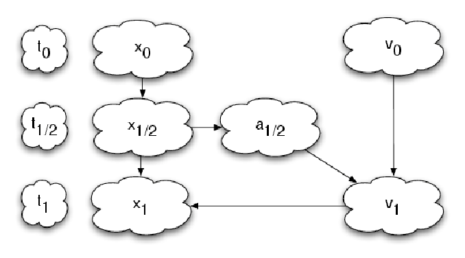
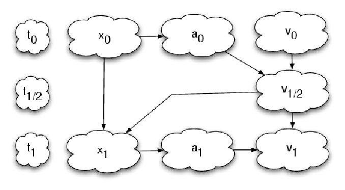
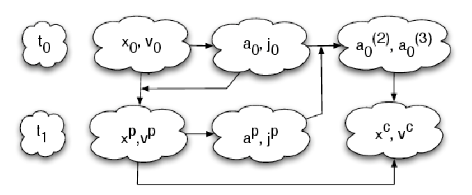
Abbildung 4: Flow charts showing the DKD leapfrog step (top) and the KDK leapfrog step (bottom).
In difference to the DKD leapfrog step, which needs only one force evaluation, the KDK leapfrog step
needs two force evaluations, which are computationally expensive. Graphics program: OMNIGRAFFLE.
Algorithms: The DKD (“Drift-Kick-Drift”) Leapfrog, also called “Position Verlet” is given by (e. g. Sutmann, 2006) DKD Leapfrog:
 2. “Kick”:
  The KDK (“Kick-Drift-Kick”) Leapfrog, also called “Velocity Verlet” is given by (e. g. Sutmann, 2006) KDK Leapfrog:
 2. “Drift”:
  Properties of leapfrogs: The leapfrog methods have the following good properties (c. f. McLachlan & Quispel, 2001):
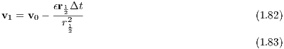
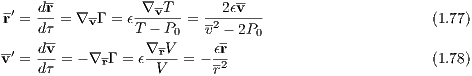
 We note that in practical computations every numerical scheme is prone to roundoff errors. For the connection to symplectic integration we refer to the work of Skeel (1999). 1.5.2 Logarithmic Hamiltonian method (LogH)The LogH method, a leapfrog with adaptive time steps is in detail described in Preto & Tremaine (1999). It is based on a so-called “functional Hamiltonian” (cf. Mikkola & Tanikawa, 1999; Preto & Tremaine, 1999; Mikkola, 2008). We introduce now a logarithmic Hamiltonian (LogH)
where 0 < ϵ ≪ 1 is an accuracy parameter and P0 is an integral of motion which equals minus the initial energy. We remark that a different functional form for the Hamiltonian can be used as well. However, it should obey the separability property with respect to x and v. In the special case of the relative motion of the two-body problem, which was treated in chapter 1, we have
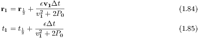
with the dimensionless relative velocity v = |v| and the dimensionless distance r = |r|. We obtain the equations of motion for the logarithmic Hamiltonian method,
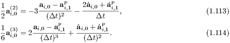
where τ is a transformed time. The time step function is given by
Preto & Tremaine (1999) remark already the nice property that the Equations (1.77), (1.78) and (1.79) do not contain any square root operations which are computationally expensive.
The DKD (“Drift-Kick-Drift”) leapfrog algorithm can, according to Preto & Tremaine (1999) and Mikkola (2008) be written as follows with an accuracy constant ϵ and an integral of motion P0 which is equal to minus the initial energy: LogH Methode / LogH method:
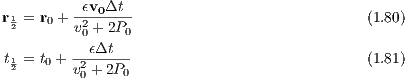 2. “Kick”:
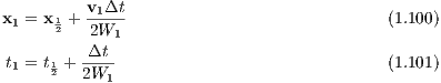
  Because of the Hamiltonian formulation the LogH method is going to preserve the two-body trajectory except for a phase error: If we integrate a two-body problem with the LogH method, the numerical solution will always stay on the corresponding conic section. The same holds for the TTL method which is discussed in the next section. 1.5.3 Time-transformed leapfrog (TTL)The TTL method, also a leapfrog with adaptive time steps is in detail described in Mikkola & Aarseth (2002) and the Cambody lecture notes by Mikkola (2008). The Hamiltonian equations of motion are given by
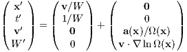
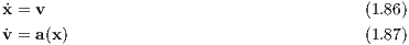 where x, v and a are position, velocity and force on a unit mass and the dot denotes a derivative with respect to time. Note that these are coupled and cannot be solved independently of each other. A time transformation
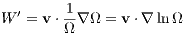
can be introduced, where Ω(x) > 0 can be the absolute value of the potential energy in the case of a few-body problem, or its square, or cube, or, for example,
We introduce an auxiliary variable W = Ω. The equations of motion in the transformed time become
 where the prime denotes a derivative with respect to the transformed time. The trick is to calculate W from the differential equation
With this trick the leapfrog scheme can be applied, since Ω = Ω(x) similar to a = a(x) and the separability property can be respected. Switching to the transformed time we obtain
We obtain the differential equations
These can be solved, for example with a DKD (“Drift-Kick-Drift”) leapfrog method. We note, however, that the separability property is not exactly realized in the equations (1.95).
The algorithm can be written as follows: TTL-Methode / TTL method:
 2. “Kick”:
  1.5.4 Higher-oder composition schemes Abbildung 6: Exact integration of the Kepler problem with an 8th-order time-transformed composition
scheme except for a phase error for an orbit with eccentricity e = 0.99. Plotting language: IDL.
Tabelle 1: Koeffizienten nach dem Theorem von Yoshida, Qin und Zhu für das Kompositionsverfahren
4. Ordnung. / Coefficients according to the theorem of Yoshida, Qin and Zhu for the 4th-order
composition scheme.
The composition schemes are higher-order leapfrog methods and in detail described in the review by Sutmann (2006). Valid is, for example, the Theorem of Yoshida, Qin and Zhu: Let
with
is a scheme of order 2n + 2 (Yoshida, 1990; Qin & Zhu, 1992), where Many other composition possibilities exist. Mathematicians try to minimize the number of computationally expensive force evaluations for a given order of the integrator. For example using the coefficients given in Table 1, Table 2 or Table 3, 4th-order, 6th-order or 8th-order composition schemes can be written in a “Position Verlet” fashion as a loop over n = 9, n = 7 or n = 15 coefficients in n = 9, n = 7 or n = 15 steps,
FOR i=1, n DO BEGIN ENDFOR1.6 Hermite integrators1.6.1 Standard Hermite method
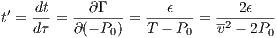
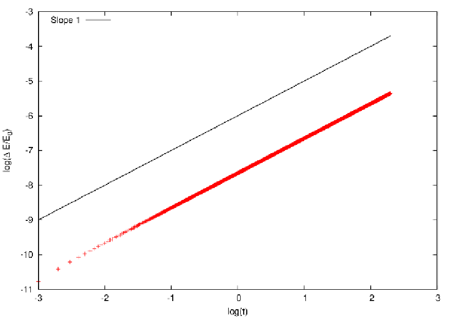
Abbildung 8: Linear growth of the relative energy error for the standard 4th-order Hermite method
for 1000 circular orbits. Plotting language: GNUPLOT.
1for (double t = 0; t < t_end; t += dt) {
2 3// Do the prediction 4 5 for (int i = 0; i < n; i++) { 6 for (int k = 0; k < 3; k++) { 7 old_r[i][k] = r[i][k]; 8 old_v[i][k] = v[i][k]; 9 old_a[i][k] = a[i][k]; 10 old_j[i][k] = jk[i][k]; 11 r[i][k] += v[i][k]*dt + a[i][k]*dt2/2 + jk[i][k]*dt3/6; 12 v[i][k] += a[i][k]*dt + jk[i][k]*dt2/2; 13 } 14 } 15 16// Calc. acc. and jerk from predicted positions and velocities 17 18 acc_and_jerk(m, r, v, a, jk, n); 19 20// Do the interpolation and correction 21 22 for (int i = 0; i < n; i++) { 23 for (int k = 0; k < 3; k++) { 24 a2[i][k] = -6*(old_a[i][k]-a[i][k])/dt2 25 - 2*(2*old_j[i][k] + jk[i][k])/dt; 26 a3[i][k] = 12*(old_a[i][k]-a[i][k])/dt3 27 + 6*(old_j[i][k]+jk[i][k])/dt2; 28 29 v[i][k] = v[i][k] + a2[i][k]*dt3/6 30 + a3[i][k]*dt4/24; 31 r[i][k] = r[i][k] + a2[i][k]*dt4/24 32 + a3[i][k]*dt5/120; 33 } 34 } 35 36// Data output 37 38 ... 39 40} Listing 1: Code fragment in C++ containing the integration loop of the
standard Hermite integrator.
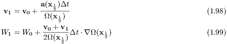
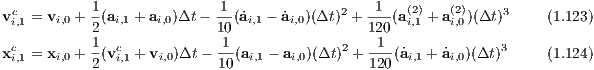
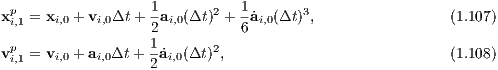
The standard 4th-order Hermite scheme (Makino, 1991; Makino & Aarseth, 1992) is in detail described in Glaschke (2006, Section 4.4) or in Ernst (2009, Section 8.2.1). It is a predictor-corrector method, which is particularly used for direct N-body simulations with N ≫ 1, since it combines the advantages of being a fast integrator and a higher-order method. We cite the latter of the above descriptions in the following subsection: Prediction step: “Positions and velocities of the ith particle are predicted according to
where the superscript ‘p’ stands for ‘predicted’ and the subscripts ‘0’ and ‘1’ for the current time t0 and the
following time t1, respectively. The acceleration ai,0 and jerk
where xji = xj - xi and vji = vj - vi are relative positions and velocities between the ith and jth
particles, respectively. Acceleration ai,1p and jerk Interpolation of higher derivatives: A second way to write down ai,1p and
Since we know the quantities Δt, ai,0,
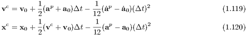
Correction step: With these quantities, positions and velocities from the prediction step can be corrected to higher orders,
 where the superscript ‘c’ stands for ‘corrected’.” (Ernst, 2009, Section 8.2.1) 1.6.2 Iterated time-symmetric Hermite method1for (double t = 0; t < t_end; t += dt) {
2 3// Do the prediction 4 5 for (int i = 0; i < n; i++) { 6 for (int k = 0; k < 3; k++) { 7 old_r[i][k] = r[i][k]; 8 old_v[i][k] = v[i][k]; 9 old_a[i][k] = a[i][k]; 10 old_j[i][k] = jk[i][k]; 11 r[i][k] += v[i][k]*dt + a[i][k]*dt2/2 + jk[i][k]*dt3/6; 12 v[i][k] += a[i][k]*dt + jk[i][k]*dt2/2; 13 } 14 } 15 16// Do the iteration 17 18 for (int l = 0; l < 3; l++) { 19 20// Calc. acc. and jerk from predicted positions and velocities 21 22 acc_and_jerk(m, r, v, a, jk, n); 23 24// Do the correction 25 26 for (int i = 0; i < n; i++) { 27 for (int k = 0; k < 3; k++) { 28 v[i][k] = old_v[i][k] + (old_a[i][k] + a[i][k])*dt/2 29 + (old_j[i][k] - jk[i][k])*dt2/12; 30 r[i][k] = old_r[i][k] + (old_v[i][k] + v[i][k])*dt/2 31 + (old_a[i][k] - a[i][k])*dt2/12; 32 } 33 } 34 } 35 36// Data output 37 38 ... 39 40} Listing 2: Code fragment in C++ containing the integration loop of the
iterated time-symmetric Hermite integrator.
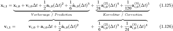
An extension is the iterated time-symmetric Hermite method (Kokubo, Yoshinaga & Makino, 1998) Prediction step: The prediction is given by
 Correction step: The corrector step is given by
 where the Hermite interpolations in Eqns. (1.113) and (1.114) have been used implicitly. Iteration: The iteration of the corrector is achieved by returning to Eqns. (1.109)–(1.110) with the predicted positions replaced by the more accurate values xc,vc (Glaschke, 2006, Abschnitt 4.5). 1.6.3 Higher-order Hermite methodsHermite mothods of higher order are explicitely described by Nitadori & Makino (2008). Prediction step: For example, the predictor for a 6th-order Hermite method is given by
Correction step: The corrector for the 6th-order Hermite method is given by
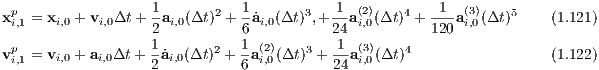
 An eighth-order method is also described in Nitadori & Makino (2008). 1.6.4 Adaptive time steps for the Hermite schemeThe standard 4th-order Hermite scheme is based on the Taylor expansions
for the ith particle, where the subscripts ‘0’ and ‘1’ stand for the current time t0 and the following time t1, respectively. The idea of adaptive time steps is as follows: Depending on the order of the integrator, its local numerical error depends usually on some positive integer power of the step width. The local error should decrease monotonically with the step width. An adaptive time step criterion adjusts the time step in such a way, that the local error remains constant or, at least, has an upper bound during the integration. Time step criteria therefore involve an estimate of the local error. Time step criteria: One may summarize a list of restrictions for the choice of an adaptive time step for the standard 4th-order Hermite integrator as follows:
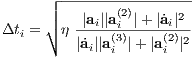
Aarseth criterion: It turns out that the Aarseth criterion
fulfills all requirements, where η is a dimensionless accuracy parameter. This criterion is well defined for
the special case ai = 0 at the Lagrangian points a tidal field or the “cold collapse” with Hierarchical block time steps: Usually one quantizes the time steps for N ≫ 1 in powers of 1∕2 such that blocks of particles with equal time steps can be integrated forwards simultaneously. 1.7 Runge-Kutta integrators (RK)The Runge-Kutta method is in detail described in Press et al. (1986). As a standard numerical integrator, it “takes an initial condition and moves the objects in the direction specified by the differential equations”. Suppose we have a system of N particles, which interact through gravity. Let mi be the mass of the ith particle and Qi,0 a 6-dimensional state vector, which contains position and velocity of the ith particle at time t0. We have then
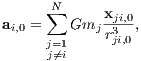
where the dot denotes the time derivative. The acceleration ai,0 obeys the Newtonian law of gravitation,
where xij,0 = xj,0 - xi,0,rij,0 = |xij,0| and the summation is over all those pairs of particles, where one of the particles is the ith particle. Of course, the ith particle does not interact with itself. Since ai,0 depends on m1,...,mi-1,mi+1,...,mN and r1,0,...,rN,0, we have a system of ordinary differential equations
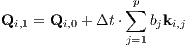
where F is the known vector mapping. Given the masses mi and the vectors Qi,0, we want to find the vector Qi,1 at time t1 = t0 + Δt, where Δt is the time step. For the pth-order Runge-Kutta mathod, we have to compute the following p 6-dimensional vectors:
with coefficients ajm given in tables 4, 5 and 6. In the above definition, F is the known vector mapping from (1.130). The integration step is then
with coefficients bj given in tables 4, 5 and 6. The coefficients for the second- and fourth-order scheme are given in Press et al. (1986). It is not known to the present author who calculated the coefficients for the eighth-order method.
Tabelle 4: Koeffizienten für das Runge-Kutta-Verfahren 2. Ordnung. / Coefficients for 2nd-order
Runge-Kutta method.
Tabelle 5: Koeffizienten für das Runge-Kutta-Verfahren 4. Ordnung. / Coefficients for 4th-order
Runge-Kutta method.
Tabelle 6: Koeffizienten für das Runge-Kutta-Verfahren 8. Ordnung. / Coefficients for 8th-order
Runge-Kutta method.
1.8 Tasks
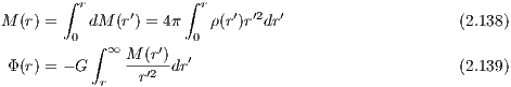
2 Galactic dynamicsThe aim of this chapter about orbital mechanics and galactic dynamics is to enable the reader to integrate orbits in different analytic gravitational potentials. It is left to the reader to write a program for the integration of orbits in these gravitational potentials. It may be useful to keep the program as general as possible to simplify the inclusion of new gravitational potentials without larger problems. 2.1 Spherically symmetric models2.1.1 Mechanical foundationsCoordinates: A spherically symmetric self-consistent model of as stellar system, which is static in time and a solution of both the Poisson and the Boltzmann equation, is given by gravitational potential Φ(r), cumulative mass M(r), density ρ(r) and velocity dispersion σ(r). These scalar quantities depend only on radius r, which is defined as the distance from the center, not from time t or velocity v. We define
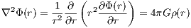
Poisson Gleichung: The Poisson equation for a spherically symmetric system is given by
where ∇2 is the Laplacian operator and G is the gravitational constant. Physical quantities: The force on a unit mass (the specific force or acceleration) is given by
where ∇ is the gradient operator. Starting from the gravitational potential, we have
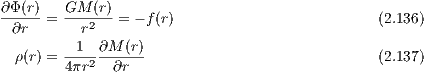 where we have used in the first step Newton’s second theorem (see Binney & Tremaine, 1987, p. 34f.) together with Newton’s law of gravitation. Starting from the density, we have
 where we assume limr→∞Φ(r) = 0 in the last step. The circular velocity vc(r) and escape velocity ve(r) are given by
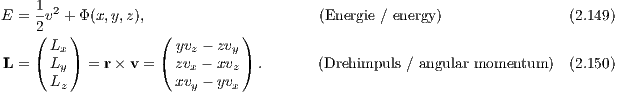
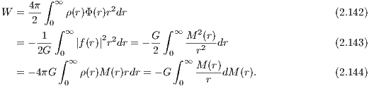
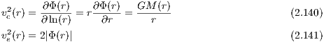 The total potential energy W is given by the equivalent expressions
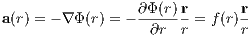
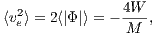
The derivation of the above integrals is discussed in chapter 2 of the book by Binney & Tremaine (1987). If the system is in virial equilibrium, the value of the potential energy W is connected to the values of total kinetic energy K = -W∕2 and the total energy E = -K = W∕2. From Eqn. (2.144) follows the root mean squared escape speed,
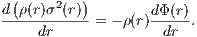
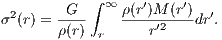
for a finite total mass M. If the velocity dispersion tensor is isotropic, we can obtain the velocity dispersion σ(r) by integrating the Jeans equation of hydrostatic equilibrium,
The velocity dispersion is given by the integral
Virial theorem: The kinetic energy due to random motion is given by the integral
where a an integration by parts has been carried out in the first step and the condition (2.146) of hydrostatic equilibrium has been plugged in in the second step. If Π is finite it follows that C = 0 and the virial theorem is fulfilled (Ernst, 2009). Integrals of motion: Two integrals of motion in static spherically symmetric stellar systems are
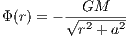
 2.1.2 Kepler potentialThe Kepler potential is solution of the Poisson equation for a point mass in the origin of coordinates and given by
Applications include, e. g., planetary dynamics or stellar orbits around a supermassive black hole. The acceleration is given by
The jerk, which is of relevance for the Hermite integration scheme, is given by 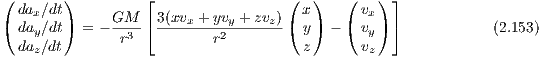 Integral of motion: An additional integral of motion in the Kepler potential is
2.1.3 Power-law models
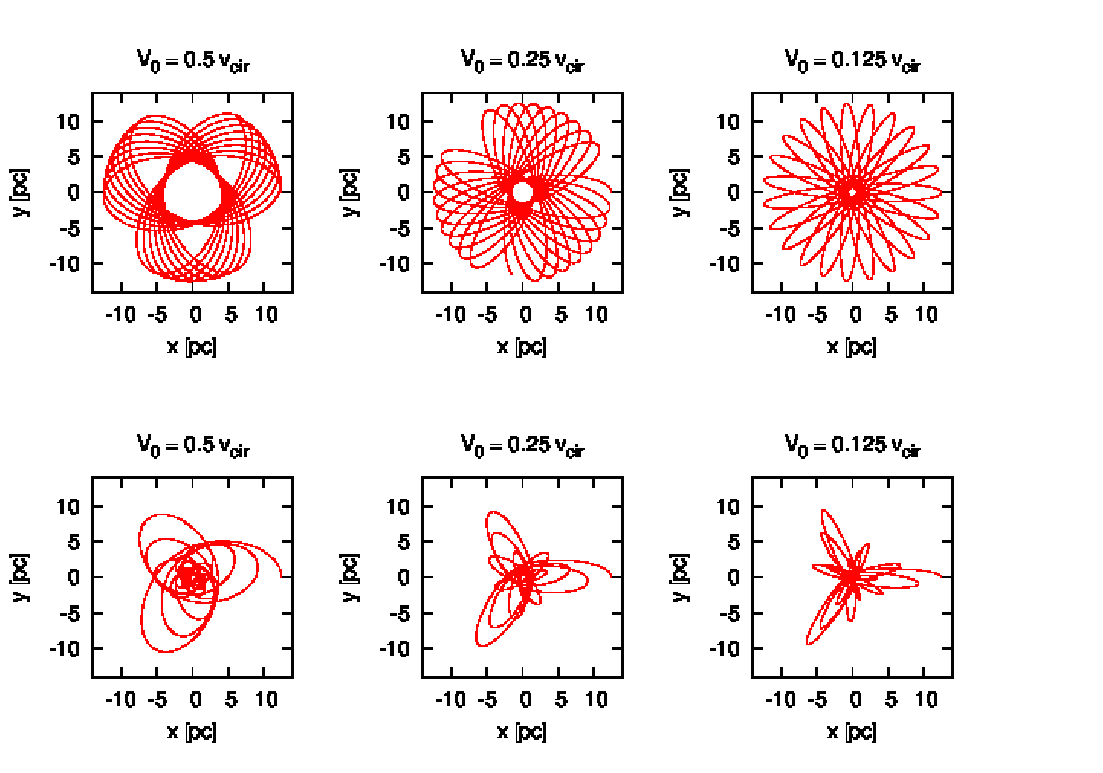
Abbildung 9: Orbits of different eccentricities in a near-isothermal sphere, a power law model with
Exponent α = 1.2. For each orbit the initial velocity is given in units of the circular velocity at the initial
galactocentric radius. Top row: Rosette orbits without dynamical friction. Bottom row: With dynamical
friction. From Ernst (2009). Integrator: INTEXT (Ernst, 2012). Plotting language: GNUPLOT.
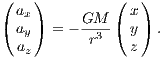
The spherically symmetric power-law or scale-free models can be used to study the dynamics in the centers of galaxies. Note that power laws are connected to self-similarity, i.e. they are scale-invariant. In particular, the models discussed below are invariant under spatial magnification. They have a potential of the form
 where r is the radius and r0 is a length unit. The acceleration has the form
The jerk is given by
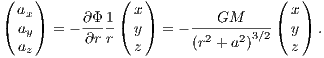
 2.1.4 Plummer modelThe gravitational potential of a Plummer model is given by
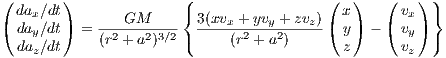
where a is the Plummer radius. The acceleration is then given by
The jerk, which is of relevance for the Hermite integration scheme, is given by
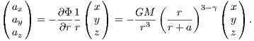
2.1.5 Dehnen modelsThe gravitational potential of a Dehnen model (Dehnen, 1993; Tremaine, 1994) has, in contrast to that of the Plummer model, a “cusp” in the center. It is given by
where a is a scale radius. The acceleration is given by
The jerk which is of relevance for the Hermite integration scheme, is given by
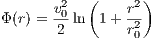
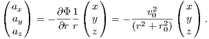
Special cases are the Hernquist model with γ = 1 (Hernquist, 1990) and the Jaffe model with γ = 2 (Jaffe, 1983). 2.1.6 Logarithmic potentialA logarithmic gravitational potential, which is often used for dark matter halos of galaxies, is given by
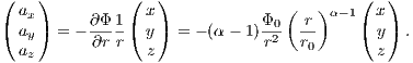
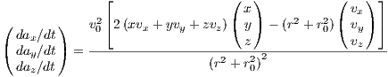
The acceleration is given by
The jerk is given by
2.2 Multi component models2.2.1 The 3PLK Milky Way model
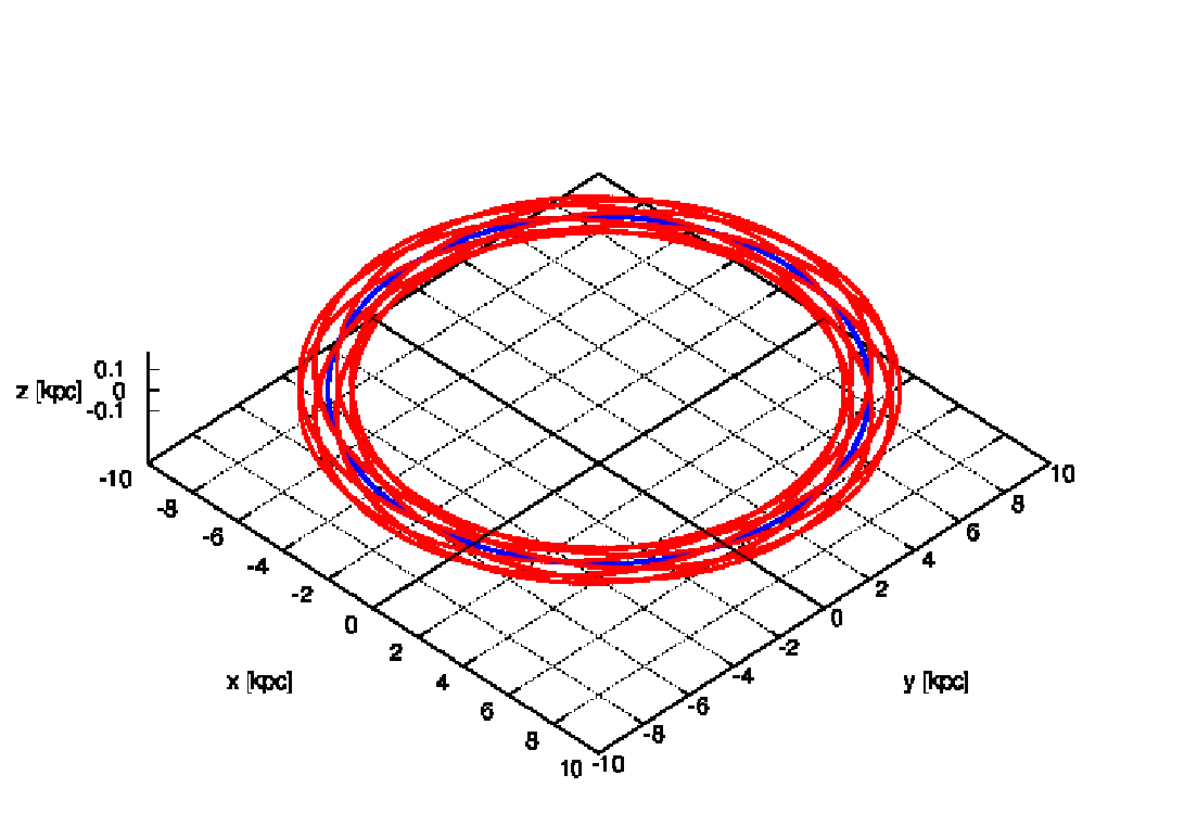
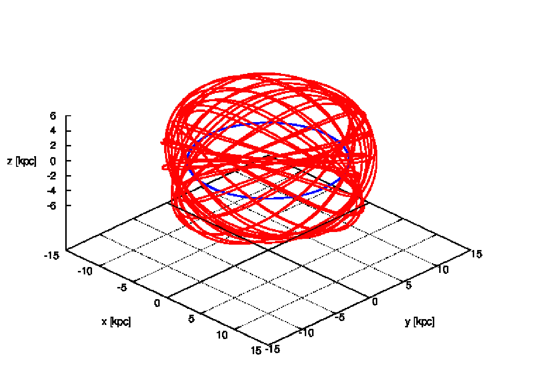
Abbildung 11: Halo orbit resembling a ball of wool for knitting socks and circular reference orbit
at the solar radius in a 3-component Plummer-Kuzmin model of the Milky Way. Integrator: INTEXT
(Ernst, 2012). Plotting language: GNUPLOT.
Tabelle 7: Die Liste der Milchstraßen-Komponenten-Parameter für das 3PLK-Modell der Milchstraße
(Peter Berczik, Patrick Glaschke). / The list of galaxy component parameters for the 3PLK model of
the Milky Way (Peter Berczik, Patrick Glaschke).
Tabelle 8: Kreisbahngeschwindigkeiten bei z = 0 an verschiendenen Galaktozentrischen Radien für
das 3PLK-Modell mit den Parametern aus Tabelle 7. Die astronomischen Konstanten sind Binney
& Tremaine (2008, Anhang A) entnommen. / Circular velocities at different galactocentric radii (at
z = 0) for the 3PLK model with the parameters of table 7. The astronomical constants are taken from
Binney & Tremaine (2008, appendix A).
The parameters of the 3-component Plummer-Kuzmin model (Miyamoto & Nagai, 1975) of the Milky Way are given in table 7.1 The total gravitational potential is given by a a superposition of three potentials for bulge, disk and halo. The circular velocity as a function of galactocentric radius is given in table 8. The gravitational potential has the form
The acceleration for the Plummer-Kuzmin model is given by the expression
The jerk is given by the lengthy expressions
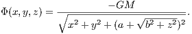
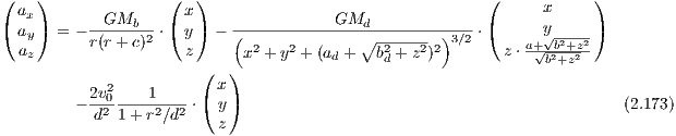
which also depend on the velocity components. A few orbits are plotted in Figures 10 and 11. 2.2.2 JSH95 Milky Way modelThe gravitational potential of the JSH95 model of the Milky Way (see Johnston, Spergel & Hernquist, 1995; Dinescu, Girard & van Altena, 1999) is given by
with Mb = 3.4 × 10¹⁰M⊙, c = 0.7 kpc, Md = 1011M⊙, ad = 6.5 kpc, bd = 0.26 kpc, v0 = 128 km s-1, d = 12.0 kpc. The bulge has a Hernquist profile, the disk is represented as a Plummer-Kuzmin model and the halo by a logarithmic potential. The acceleration for the JSH95 model is given by the expression
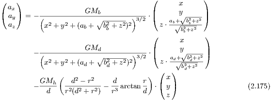
2.2.3 P90 Milky Way modelThe gravitational potential of the P90 model of the Milky Way (see Pacyński, 1990; Dinescu, Girard & van Altena, 1999) is given by
![GMb GMd
Φ(r) = - ∘-------------∘---------- ∘---------------∘--------
x2 + y2 + (ab + z2 + b2b)2 x2 +y2 + (ad + z2 + b2d)2
GMh [1 ( r2) d r]
+ --d-- 2 ln 1+ d2 - r arctan d (2.174)](simplyhtml154x.png) with Mb = 1.12 × 10¹⁰M⊙, ab = 0.0 kpc, bb = 0.277 kpc, Md = 8.0710M⊙, ad = 3.7 kpc, bd = 0.20 kpc, Mh = 5 × 10¹⁰M⊙, d = 6.0 kpc. The acceleration for the P90 model is given by the expression
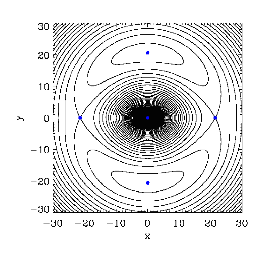
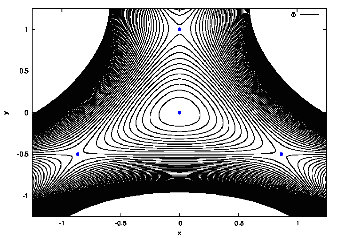
2.2.4 Zotos’ barred spiral galaxy model Abbildung 12: The effective potential of a barred spiral galaxy from Eqn. (2.176) in 2D. The contours
are the isolines of constant effective potential. The positions of the Lagrangian equilibrium points L1
- L5 are marked with blue dots. Plotting language: IDL.
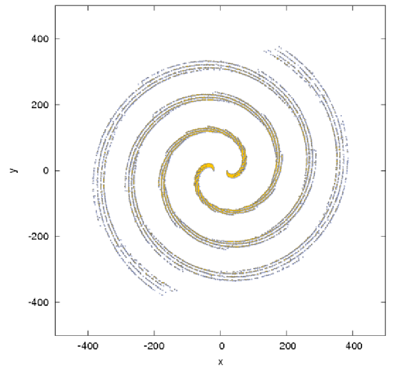
Abbildung 13: Forming spiral arms of a grand-design spiral in the effective potential in Eqn. (2.176).
The density of points along one orbit is taken to be proportional to the velocity as described in Ernst
& Peters (2014). Plotting language: GNUPLOT. Post-processed with GIMP.
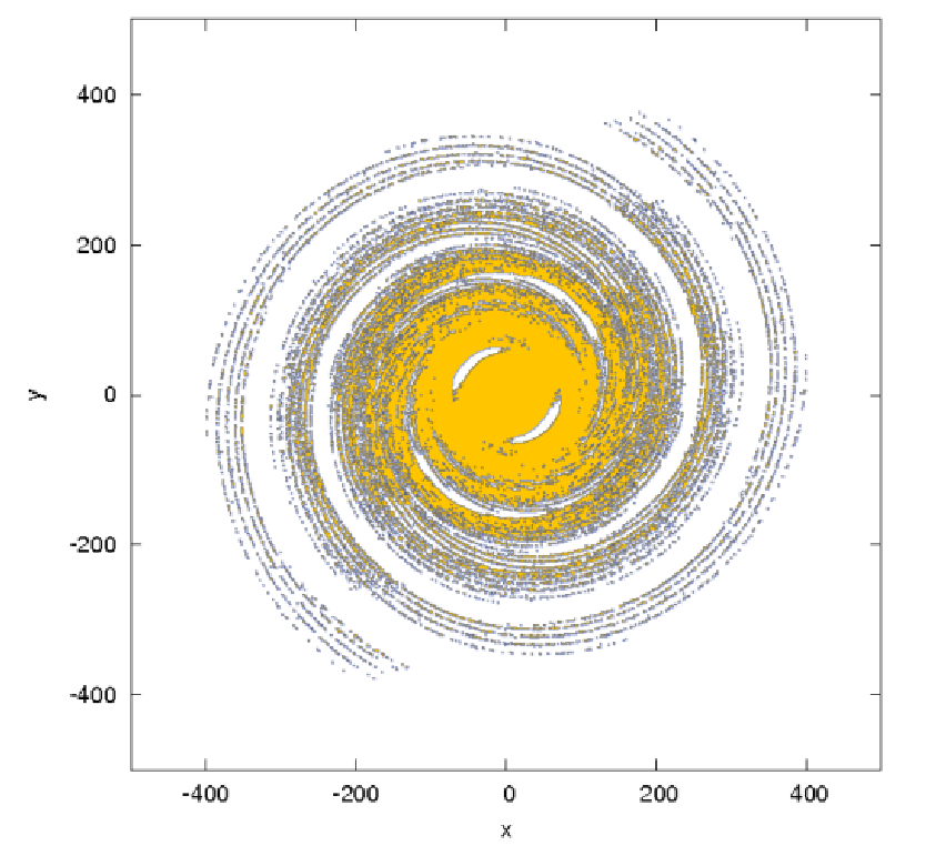
Abbildung 14: Fully-fledged spiral arms in the effective potential in Eqn. (2.176). The density of
points along one orbit is taken to be proportional to the velocity as described in Ernst & Peters (2014).
Plotting language: GNUPLOT. Post-processed with GIMP.
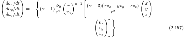
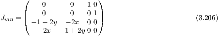
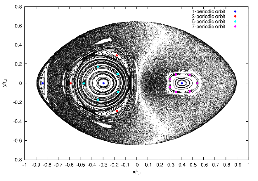
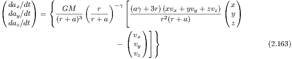
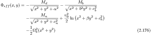
The simple 2D effective potential of a barred spiral galaxy according to Zotos (2012), which is visualised in Figure 12, is given by the terms
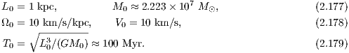
with the parameters α = 8, β = 1.3, b = 2, v0 = 15, Md = 9500, Mb = 3000, Mn = 400, cb = 1.5, cn = 0.25 and ch = 8.5. We have Ωb = 1.25. The model consists of a logarithmic halo, a disc, a Plummer nucleus (bulge) and a bar. The potential rotates clockwise at constant angular velocity Ωb. The effective potential in Eqn. (2.176) is the cut through the equatorial plane of a typical 3D potential of a barred spiral galaxy. We remark that for a axisymmetric halo the parameter β should be set to β = 1. In Eqn. (2.176), the model units of length L0, velocity V 0, angular velocity Ω0, time T0 and mass M0 of the parameters, in which the gravitational constant G = 1, can be scaled to physical units of a realistic barred spiral galaxy as NGC 1300:
The equations of motion in the rotating frame are given by
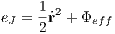
where r = (x,y,z) is the position vector, the dot denotes a derivative with respect to time and Φ is given by the first four terms in Eqn. (2.176). The Jacobi energy is an integral of motion and given by
A critical Jacobi energy is given by the value of the effective potential Φeff at the position of the two saddle points in Figure 12. Figures 13 and 14 illustrate fully-fledged spiral arms, which have been formed in the potential of Eqn. (2.176), as described in Ernst & Peters (2014). The spiral arms form out of escaping particles with overcritical Jacobi energies. The density of points along one orbit in figures 13 and 14 is taken to be proportional to the velocity of a particle. This method can be called the “velocity-dependent plotting technique”. The spiral galaxies in this theory display spiral patterns which are persistent in time, in contrast to the transient spiral patterns in the old density wave theory (e.g. Pasha, 2004a,b). The winding problem in differentially rotating disks does not occur (“Weizsäcker’s cow”). Also, a large number of different galaxy morphologies can be reproduced in this theory. 2.3 Tasks
3 Linear stability analysis3.1 Introduction to linear stability analysisThe linear stability analysis of equilibria is an important part of nonlinear dynamics. For this purpose one linearizes the dynamics around the equilibrium and considers the dynamics in this linearized theory, which is simpler than the full nonlinear theory. Methods of linear algebra are used. A German reference for linear algebra are the two books by Lorenz (1992a,b). In particular, the eigenvalue problem for the Jacobi matrix must be solved. One-dimensional systems: Let
be a one-dimensional (1D) map. The Jacobi matrix consists of only one element,
If the modulus of the derivative, is smaller than one (larger than one) the corresponding fixed point is stable (unstable). If it is equal to one, we speak of a marginally stable fixed point. Two-dimensional systems: Let, in a two-dimensional (2D) system,
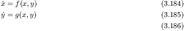 The Jacobi matrix is given by
We can classify equilibrium points in two dimensions (2D) as follows (e. g. Izhikevich, 2007):
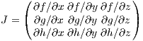
Three-dimensional systems: Let, in a three-dimensional (3D) system,
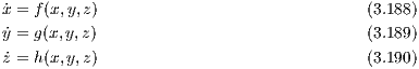 The Jacobi matrix is given by
We can classify equilibrium points in three dimensions (3D) as follows (e. g. Izhikevich, 2007):
3.2 Logistic Map (1D)
1//--------------------------------------------------------------
2// feigenbaum.C 3// Code: Calculates Feigenbaum diagram for logistic map 4// Author: Andreas Ernst 5// Date: August 8, 2006 6//-------------------------------------------------------------- 7 8#include <iostream> 9#include <cmath> 10#include <cstdlib> 11 12using namespace std; 13 14int main() { 15 16 double h = 0.001, h0=0.001; 17 double x; 18 int niter = 1000; 19 20 for (double lambda=0.25; lambda<=3; lambda+=h) { 21 for (double x0=h0; x0<=1; x0+=h0) { 22 x = x0; 23 for (int n=1; n<=niter; n++) { 24 x = 4*lambda*x*(1-x); 25 if (n==niter) cout << lambda << "␣␣␣" << x << endl; 26 } 27 } 28 } 29 return 0; 30} 31//-------------------------------------------------------------- Listing 3: C++ code feigenbaum.C for the Feigenbaum diagram
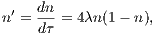
History: Historically, the non-linear logistic equation
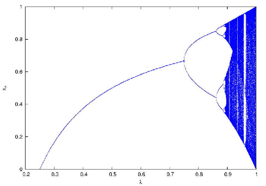
here with a free parameter λ, was introduced by Pierre-François Verhulst for studying population dynamics (Verhulst, 1838). The solutions for n(τ) < 1 are characteristic S-shaped curves, so-called sigmoid functions. Logistische Abbildung: The associated discrete logistic map is given by
with a free parameter λ. A plot of xn vs. λ for a large n yields the so-called Feigenbaum diagram shown in Figure 15. By increasing λ, it can be seen that at the period doubling bifurcations the fixed point(s) get(s) unstable. This is the “route into chaos”. Linear stability analysis: The Jacobi matrix element is given by
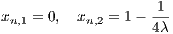
For a fixed point we have the condition
We obtain two solutions,
We find
3.3 Hénon-Heiles system (2D)
Abbildung 16: Equipotential lines for the Hénon-Heiles potential. The equilibrium points are marked
with blue dots. Plotting language: GNUPLOT.
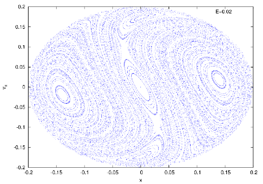
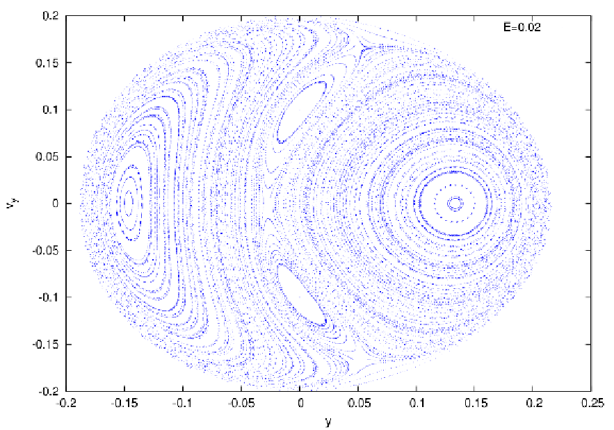
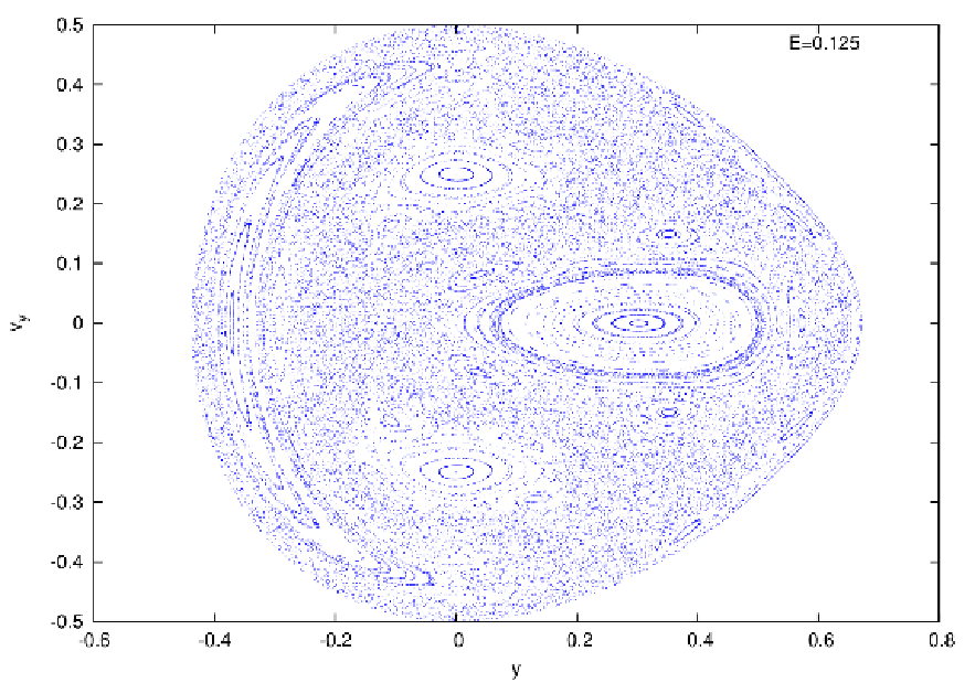
Abbildung 17: Poincaré surfaces of section in the Hénon-Heiles potential with x = 0 and vx ≥ 0. Top
panel: At E = 0.02. We see only periodic and quasiperiodic orbits. Bottom panel: At E = 0.125. We
see a mixture of periodic, quasiperiodic and chaotic orbits. Plotting language: GNUPLOT.
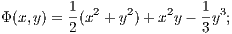
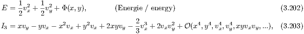
History: Historically, the Hénon-Heiles system was the first system for which the existence of a so-called adelphic or non-classical integral of motion was demonstrated numerically. Figure 16 shows that the potential is not axisymmetric but has only a triangular symmetry according to the dihedral group D3 (Cushman, 2005). Hence the z-component of angular momentum is only approximately conserved. The energy is conserved exactly since the Hénon-Heiles system is a Hamiltonian system. The adelphic integral of the Henon-Heiles system can be represented as a power series, whose lowest order is the z-component of angular momentum (Finkler, Jones & Sowell, 1990). The Hénon-Heiles potential (Hénon & Heiles, 1964) is given by
Figure 16 shows the equipotential lines. The potential has a minimum H1 and three saddle points H2, H3 and H4. Equations of motion: The equations of motion are
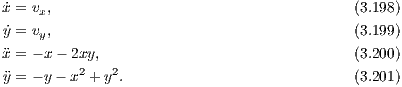 Figure 17 shows two Poincaré surfaces of section at two different energies. In the top panel of Figure 17 all orbits are quasiperiodic or periodic. In the bottom panel of Figure 17 there are large dotted chaotic regions in which smaller quasiperiodic islands are embedded. Integrals of motion: The integrals of motion are
where I3 is the adelphic integral to third order (Finkler, Jones & Sowell, 1990). Linear stability analysis: Equilibrium points are determined via
The solutions are
The central potential is Φ(H1) = 0. The potential at the saddle points is Ecrit = Φ(H2) = Φ(H3) = Φ(H4) = 1∕6. For energies E > Ecrit particles can escape from the central region of the potential. We proceed with a linear stability analysis. The Jacobi matrix is given by
 We consider the 2 × 2 submatrix of J,
 The characteristic polynomial is given by
The general solutions are given by
We find:
Computation of Poincaré surfaces of section: Interpretation of Poincaré surfaces of section: Algorithm for finding periodic orbits on a Poincaré surface of section:
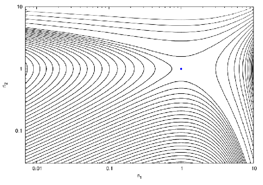
3.4 Lotka-Volterra system (2D)Population dynamics: Assume a system, in which two species interact, the predator and the prey populations. In the field of astrophysics at the university, the predator species might be the astrophysicists and the prey “species” the public funds (not: third-party funds). The theory of such a system is well-known and can near the fixed points be described by a system of coupled differential equations, the Lotka-Volterra equations,
where the variables are defined as follows:
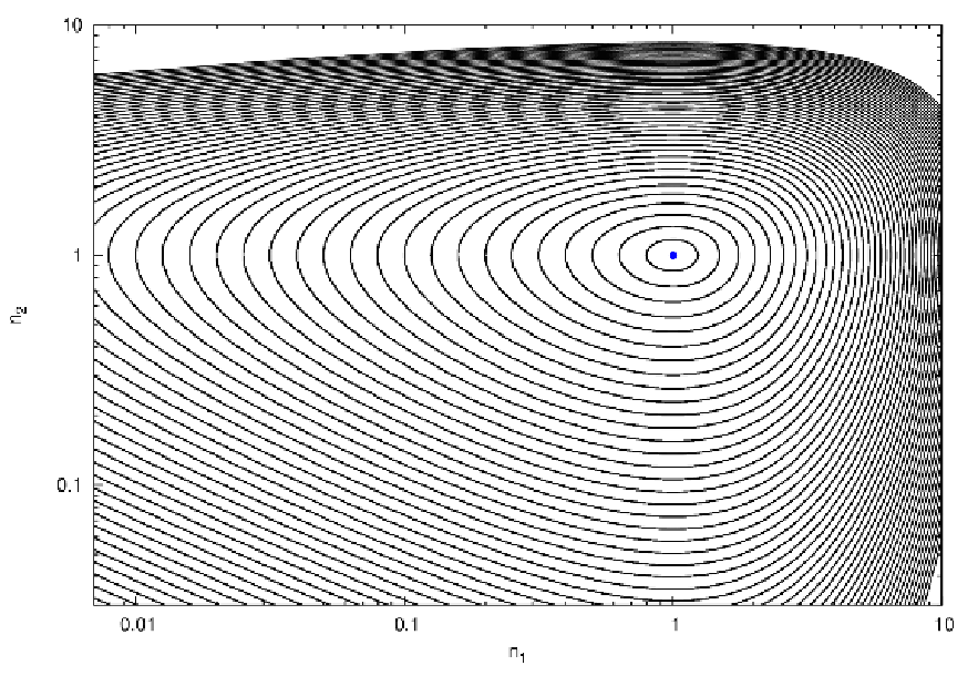
Abbildung 18: Top panel: Phase portrait for Eqns. (3.215) and (3.216) for λ = 0.5. A marginally
stable fixed point at (n1,n2) = (1,1) can be seen. n1 and n2 have upper and lower limits. Bottom
panel: Phase portrait for Eqns. (3.215) and (3.216) for λ = -0.5. The fixed point at (n1,n2) = (1,1)
is unstable and n1 and/or n2 die out or grow infinitely in number. The position of the fixed point is
marked with a blue dot in both panels. Plotting language: GNUPLOT.
Dimensionless formulation: We may introduce scaled variables (e. g. Kühn & Spurzem, 2005),
 to arrive at the dimensionless formulation
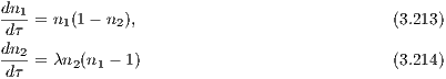
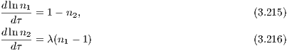
with only one free parameter λ. In logarithmic notation, Eqns. (3.213) and (3.214) can be written more concisely as
Solutions: Figure (18) shows phase portraits for the Eqns. (3.213) - (3.214). These are similar to the Poincaré surfaces of section except for the fact that the solutions of the Eqns. (3.213) - (3.214) are all regular (non-chaotic), such that the phase can be identified easily. One solution is shown in Figure 19 for λ = 0.5. Linear stability analysis: For stationary solutions we set the left-hand sides of Eqns. (3.213) and (3.214) to zero,
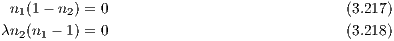 The solutions for arbitrary λ are
For λ = 0 other solutions exist. We proceed with a linear stability analysis. For that purpose we consider the Jacobi matrix
with m = 1,2 and n = 1,2. The eigenvalues are given by the zeros of the characteristic polynomial, i.e.
The general solutions are given by
The stability of the fixed point E1 can be seen as follows: At E1 the solutions are
We have Re
The top panel of Figure 18 shows that for λ = 0.5 these eigenvectors point indeed in the right direction at E1, i.e. that they are parallel to the n1 and n2 axes, respectively. 3.5 Lorenz attractor (3D)
Abbildung 20: Top panel: The Lorenz attractor for σ = 10,b = 8∕3,r = 28. Bottom panel: The
Rössler attractor for a = 0.15,b = 0.20,c = 10. Plotting language: R.
History: Edward N. Lorenz was a meteorologist working on the theory of the weather. “He reduced the Navier-Stokes equations in the Boussinesq approximation for a plane, from below heated fluid model [...] to a system of three ordinary nonlinear differential equations, which governs the temporal evolution of three fundamental modes, a velocity and two temperature distributions” (Argyris, Faust & Haase, 1995). Equations of motion: The system of equations of motion for the Lorenz attractor (Lorenz, 1963) are given by
Solution: They describe a so-called “strange attractor” (Ruelle & Takens, 1971), which is shown in the upper panel of Figure 20. A possible choice of the parameters is σ = 10, b = 8∕3, r = 28. Linear stability analysis: The Jacobi matrix is given by
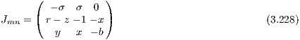 The fixed points are for b ⁄= 0 given by
The Jacobi matrix at L1 is given by (cf. Argyris, Faust & Haase, 1995)
 The eigenvalues of JL1 are given by
We find that
3.6 Rössler attractor (3D)History: Otto E. Rössler searched for a simpler “strange Attractor” than the Lorenz attractor. He found one. Equations of motion: The system of equations of motion for the Rössler attractor (Rössler, 1976) are given by
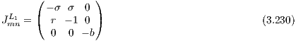
Solution: The lower panel of Figure 20 shows the Rössler attractor. A possible choice of the parameters is a = 0.15, b = 0.20, c = 10. Linear stability analysis: The Jacobi matrix is given by
 The fixed points are for a ⁄= 0 given by
The Jacobi matrix at R1 is given by
 The characteristic polynomial at R1 is given by
The eigenvalues of JR1 are given by
We find that
3.7 Tasks
4 Integrating the stellar initial mass function
Abbildung 21: The Kroupa (2002) initial mass function, a segmented power law. Plotting language:
GNUPLOT.
More information can be found in the book “An introduction to the Theory of Stellar Structure and Evolution” by D. Prialnik (Prialnik, 2000). According to Salpeter (1955), the initial mass function ξ(m) (IMF) is defined as the number of stars per unit logarithmic mass interval, or, equivalently, as “the amount of mass in stars with masses in the interval [m,m + dm] formed at a given time in a given volume of space”,
where m = M∕M⊙ is the mass in solar mass units and the IMF is assumed to be a simple power law. Salpeter found a single power law index of
for stars in the solar neighborhood. However, the lower and upper bounds of stellar masses dictated by the laws of stellar structure and evolution imply that the Salpeter IMF is not scale free as the power law (4.240) with the exponent (4.241) suggests. One may as well define a function ϕ(m), which is sometimes called the “stellar birth function”, as the number of stars per unit mass interval, or, equivalently, the number of stars with masses in the range [m,m + dm] formed at a given time in a given volume of space,
Kroupa, Tout & Gilmore (1993) found the following double-logarithmic slopes of the IMF (4.240):
where the most drastic change in the power law index at 0.5 M⊙ may indicate the existence of a characteristic mass scale in the star formation process, as Kroupa et al. notice. However, the IMF given by (4.243) is a relation which has been found empirically for stars in the solar neighborhood. The slope for the higher-mass stars (above one solar mass including the whole upper main sequence), is slightly higher than the Salpeter slope (4.241). In Kroupa (2002), the IMF is extended to the very low mass regime:
The 4 constants in (4.244) are obtained by solving the system of 4 linear equations,
4.1 Integral solvingTo obtain the result in Eqn. (4.245) we need to evaluate the corresponding integral. This can be done analytically for the case of the Kroupa (2002) IMF in Eqn. (4.244) or numerically. For the numerical computation, there are three main approaches: 4.1.1 Solving a differential equationWe may solve the corresponding differential equation (see e. g. Press et al., 1986),
for N = y(120.0) with the boundary condition y(0.01) = 0. For this purpose, we may use an appropriate integrator, e. g. a Runge-Kutta method. 4.1.2 Using geometrical rulesWe may use geometrical rules such as the trapezoidal rule (see e. g. Press et al., 1986):
with the step size 0 < h ≪ 1. Higher-order geometrical rules are the Simpson’s rule, Simpsons 3∕8 rule or Bode’s rule (see e. g. Press et al., 1986). 4.1.3 Monte-Carlo integrationWe need a suitable majorizing function Φ(m) of the function ϕ(m) with ϕ(m) < Φ(m) in the whole integration interval, whose integral is known. Now we “sprinkle” the area in the integration range below the majorizing function with random points. The knowledge of the ratio of the number of points below the function ϕ(m) and the number of points below the majorizing function Φ(m) allows the determination of the integral. We note that majorizing integrability is connected to the mathematical possibility to exchange integration and limiting procedure. 4.2 Tasks
5 Astrophysical Poisson equationsThis chapter is based on lectures and exercises by Prof. W. M. Tscharnuter at the University of Heidelberg. The theory of the Lane-Emden equation can be found in the book “Galactic dynamics” of J. Binney and S. Tremaine (Binney & Tremaine, 1987, 2008). 5.1 Lane-Emden equationThe polytropic equation of state is
where K is the polytropic constant, n is the polytropic index and P and ρ are pressure and density, respectively. An integration of the equation of hydrostatic equilibrium
where Φ is the gravitational potential, leads to
The Poisson equation reads then
Introducing dimensionless quantities s and ψ(s),
![ψ(s) =-Φ-, (5.253)
Φc
s = (- Φc )(n-1)∕2Ar, (5.254)
4πG
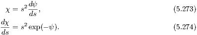
A2 = [(n+-1)K-]n-, (5.255)](simplyhtml231x.png) we obtain the Lane-Emden equation
which has analytical solutions for n = 0,n = 1 and n = 5. For other values of n, it must be solved numerically using the boundary conditions ψ(z = 0) = 1, which means that the central potential is finite and dψ∕ds|s=0 = 0, which corresponds to a flat core of the stellar polytrope. To integrate it, we replace it into a system of two first-order differential equations,
 The solutions are shown in Figure 22. 5.1.1 Chandrasekhar massFrom (5.251) follows a relation between central potential Φc and central density ρc,
and we have
On the other hand, from (5.251) and (5.259) follows
Solving (5.260) for ρc yields
We now have for the cumulative mass
|In addition to the dimensionless constant Mn = - Plugging in (5.262) in (5.266), we obtain after some tedious calculation the important relation
between the polytropic constant K, the radius R and the cumulative mass M. Solving for the polytropic constant K and plugging it in the polytropic equation of state (5.249), we find
For the case n = 3 (relativistic degenerate electron gas), we find for the central pressure
where G is the gravitational constant and the numerical constant M3 ≈ 2.01824. On the other hand, quantum statistics of a relativistic degenerate electron gas tells us that
where h,c,mp are the Planck constant, the speed of light and the proton mass, respectively, and μe = 2. Equating these two and solving for the mass gives the famous Chandrasekhar mass
5.1.2 Isothermal case
Abbildung 23: Regular and singular solutions of the isothermal Lane-Emden equation and Taylor
expansion which covers the core of the regular solution. Plotting language: GNUPLOT.
Abbildung 24: Gravitational potential of the isothermal sphere and limiting cases. Plotting language:
GNUPLOT.
Abbildung 25: Existence of the Jeans mass of an isothermal sphere. The maximum is at θ ≈ 14.
Plotting language: GNUPLOT.
Abbildung 26: UV-diagram (“isothermal curl”). Note the similarity with the proboscis of a butterfly
which is flying over the meadows in springtime. Plotting language: GNUPLOT.
The corresponding equation for the isothermal sphere is given by
Their corresponding system of first-oder differential equations is given by
 Illustrations of the solutions are shown in Figures 23, 24, 25 and 26. 5.2 Tasks
Afterword The author would like to thank Dr. Thomas Peters for helping out with calculations and Dr. Patrick Glaschke for teaching him the “high art” of theoretical physics. Furthermore, the author would like to thank Prof. Dr. Rainer Spurzem and Prof. Dr. Andreas Just. For the method of writing bilingual scripts the author is grateful to Prof. Dr. em. Franz Wegner at the University of Heidelberg. Last, the author would like to thank Prof. Dr. em. Werner M. Tscharnuter for interesting lectures on celestial mechanics in the winter term 2006/2007 at the University of Heidelberg from which some of the material presented here stems. The present book would not be without the existence of the stellar dynamics working group at the Astronomisches Rechen-Institut in Heidelberg, Germany, led by Prof. Dr. Rainer Spurzem and Prof. Dr. Andreas Just, their vivid exchange of knowledge with Dr. Sverre Aarseth at the Institute of Astronomy in Cambridge, UK (you may also read the book by Aarseth, 2003), and the possibility of being involved for years in this interesting field of research, which is beyond the mainstream topics of modern physics. The author hopes, that the tradition of doing N-body calculations at the Astronomisches Rechen-Institut, which once started with Dr. Sebastian von Hoerner (you may also read the article by von Hoerner, 2001) continues to be pursued in the future. And your life, dear reader, and mine, how shall they be pursued? I dreamed: ... La vie, la route des routes ... On my balcony grows a tiny beech tree in a blue plastic bucket. Did a bird deposit a beechnut in the bucket for hard times? Or is it going to be a blackberry bush? How is it possible to comprehend this sprouting, growing, blossoming, maturing, reproducing, prospering and lastly dying life in its entirety? I think of Hanna’s words to the Homo Faber: »You do not treat life as a living shape, but as a mere addition, therefore no relation to time, because no relation to death. Life is living shape in time.« ReferencesAarseth S. J., 1985, in: Brackbill J. U. and Cohen B. I., eds., 1985, Multiple Time Steps, Academic Press, New York, p. 377. Aarseth S. J. 1999, PASP, 111, 1333 Aarseth S. J. 2003, Gravitational N-body simulations – Tools and Algorithms, Cambridge University Press, Cambridge, UK Argyris J., Faust G., Haase M., 1995, Die Erforschung des Chaos, Vieweg Verlag, Deutschland Binney S., Tremaine S., 1987, Galactic dynamics, Princeton University Press, Princeton, USA Binney S., Tremaine S., 2008, Galactic dynamics, second edition, Princeton University Press, Princeton, USA Blanchet L., 2006, Living Rev. Relativity, 9, 4 Broucke C., 2002, AIAA 2002, 4544 Burrau C., 1913, Numerische Berechnung eines Spezialfalles des Dreikörperproblems, Astron. Nachr. 195, 113 Chencincer A., Montgomery R., 2000, Annals of Mathematics, 151, 881 Contopoulos G., 2002, Order and Chaos in Dynamical Astronomy, Springer, Berlin, Heidelberg, Deutschland Cushman R., 2005, No Polar Coordinates. Lectures by Richard Cushman., in: Efstathiou K., Sadovskií D., eds., Geometric Mechanics and Symmetry: the Peyresq Lectures, London Mathematical Society Lecture Note Series, No. 306, Cambridge University Press, Cambridge, UK, p. 211 Dehnen W., 1993, MNRAS, 265, 250 Dinescu D. I., Girard T. M., van Altena W. F., 1999, AJ, 117, 1792 Ernst A., 2009, Dissertation, University of Heidelberg, Deutschland, http://www.ub.uni- heidelberg.de/archiv/9375 Ernst A., 2012, NBODY6TID manual, http://www.simplyintegrate.de Ernst A., Peters T., 2014, MNRAS, 443, 2579 Finkler P., Jones E. C., Sowell G. A., 1990, Phys. Rev. A, 42, 1931 Gadamer H.-G., 1990, Wahrheit und Methode. Grundzüge einer philosophischen Hermeneutik., 6. Auflage, J. C. B. Mohr (Paul Siebeck), Tübingen, Deutschland Gasiorowicz S., 1996, Quantum Physics, second edition, Wiley & Sons Glaschke P., 2006, Dissertation, University of Heidelberg, Deutschland, http://www.ub.uni-heidelberg.de/archiv/6553 Green S. F., Jones M. H., eds., 2003, 2004, An introduction to the sun and stars, The Open University, Cambridge University Press, Cambridge, UK Heggie D. C., Mathieu R. D., 1986, in Hut P., McMillan S., eds., LNP 267, The Use of Supercomputers in Stellar Dynamics Standardised Units and Time Scales, Springer Verlag, Berlin, p. 233 Hempel C. G., 1977, Aspekte wissenschaftlicher Erklärung, de Gruyter, Berlin, New York Hénon M., Heiles C., 1964, Astron. J., 69, 73 Hénon M. 1976, Cel. Mech. Dyn. Astron., 13, 267 Hernquist L., 1990, Ap. J. 356, 359 v. Hoerner S., 2001, How it All Started, in: Deiters S., Fuchs B., Just A., Spurzem R., Wielen R., eds., Dynamics of Star Clusters and the Milky Way, ASP Conference Series, Vol. 228 Eugene M. Izhikevich (2007), Scholarpedia, 2(10):2014 with small changes by the present author Jaffe W., 1983, MNRAS, 202, 995 Johnston K. V., Spergel D. N., Hernquist L., 1995, Ap. J., 451, 598 Just A., Peñarrubia J. 2005, A&A, 431, 861 Just A., Khan F. M., Berczik P., Ernst A., Spurzem R., 2011, MNRAS 411, 653 Kokubo E., Yoshinaga K., Makino J., 1998, MNRAS 297, 1067 Kühn R., Spurzem R., 2005, Introduction to Computational Physics, Vorlesungsskript, Universität Heidelberg, Deutschland Kroupa P., Tout C. A., Gilmore G., 1993, MNRAS, 262, 545 Kroupa P., 2002,. Science, 295, 82 Kuypers F., 1997, Klassische Mechanik, 5. Auflage, Wiley-VCH, Weinheim, Deutschland Li, T.-Y., Yorke, J. A.,1975, The American Mathematical Monthly, 82, p. 985 Lorenz E. N., 1963, J. of the athmospheric sciences, 20, 130 Lorenz F., 1992, Lineare Algebra I, B.I. Wissenschaftsverlag, Mannheim, Leipzig, Wien, Zürich Lorenz F., 1992, Lineare Algebra II, B.I. Wissenschaftsverlag, Mannheim, Leipzig, Wien, Zürich McLachlan R., 1995, SIAM J. Sci. Comp., 16, 151 McLachlan R., Quispel R., 2001, Six Lectures on the Geometric Integration of ODEs, in: DeVore R., Iserles A., Süli E., eds., Foundations of Computational Mathematics, Cambridge University Press, Cambridge, UK, p. 155 Makino J., 1991, Ap. J., 369, 200 Makino J., Aarseth S. J., 1992, PASJ, 44, 141 Martynova, A. I., Orlov V. V., 2009, Astron. Lett., 35, 572 McLachlan R., 1995, SIAM J. Sci. Comp., 16, 151 Moore C., 1993, Phys. Rev. Lett., 70, 3675 Mikkola S., Tanikawa K., 1999a, MNRAS, 310, 745 50 Mikkola S., Tanikawa K., 1999b, Cel. Mech. Dyn. Astron., 74, 287 Mikkola S., Aarseth S. J., 2002, Cel. Mech. Dyn. Astron., 84, 343 Mikkola S., 2008, in: Aarseth S., Tout, C., Mardling R., eds., The Cambridge N-body lectures, Lecture Notes in Physics, Volume 760, Springer Verlag, Berlin, Heidelberg, Deutschland Miyamoto M., Nagai R., 1975, PASJ, 27, 533 Nitadori K., Makino J., 2008, New Astronomy, 13, 498 Ouyang T., Xie Z., arXiv:1306.0119v2 Paćynski B., 1990, Ap. J., 348, 485 Pasha I. I., arXiv:arXiv:astro-ph/0406142 Pasha I. I., arXiv:astro-ph/0406143 Peetre J., 1997, Ernst Meissel and the Pythagorean problem - the Drei-Körper-Problem in the Nachlass Meissel Plummer H. C., 1911, MNRAS 71, 460 Ruelle D., Takens F., 1971, Commun. Math. Phys., 20, 167 Press W. H., Flannery B. P., Teukolsky S. A., Vetterling W. T., 1986, Numerical Recipes - The Art of Scientific Computing, Cambridge University Press, Cambridge, UK Preto M., Tremaine S. 1999, AJ, 118, 2532 Prialnik D., 2000, An Introduction to the Theory of Stellar Structure and Evolution, Cambridge University Press, Cambridge, UK Qin M., Zhu W. J., 1992, Computing, 27, 309 Regenbogen A., Meyer U., Hrsg., 2013, Wörterbuch der philosophischen Begriffe, Felix Meiner Verlag, Hamburg, Deutschland Rössler O., 1974, Phys. Lett., 57A, 397 Salpeter E. E., Ap. J., 121, 161 Simó C., 2000, Dynamical properties of the figure eight solution of the three-body problem, Proceedings of thr ECM, Barcelona, http://www.maia.ub.es Skeel R. D., 1999, Appl. Num. Math., 29, 3 Spurzem R., 1999, J. Comp. Appl. Maths, 109, 407 Sundman K. F., 1912, Acta Math., 36, 105 Sutmann G., 2006, Molecular dynamics - Vision and Reality, in: Grotendorst J., Blügel S., Marx D., eds., Computational Nanoscience - Do it yourself!, Lecture Notes, NIC Series Volume 31, Forschungszentrum Jülich, Deutschland Šuvakov M., Dmitrašinović V., 2013, arXiv:1303.0181v1 Szebehely V., Peters C.F., 1976, Astron. J., 72, 876 Tremaine S. et al., 1994, AJ, 107, 634 Vanderbei R. J., 2004, Ann. of the New York Academy of Sciences, 1017, 422, arXiv:astro-ph/0303153 Verhulst P. F., 1838, Notice sur la loi que la population poursuit dans son accroissement., Corresp. Math. Phys.. 10, 113-121 Verlet L., 1967a, Phys. Rev. 159, 98 Verlet L., 1967b, Phys. Rev. 165, 201 Wikipedia, the English-German dictionary of the LEO GmbH (http://dict.leo.org) as well as the Wörterbuch der philosophischen Begriffe of the Meiner Edition (Regenbogen & Meyer, 2013) have been used as further sources of information. A Solutions and hints for some exercises
Abbildung 27: Time evolution of the relative energy error for the iterated time-symmetric Hermite
method for 1000 circular orbits in dependence of the number of iterations. Plotting language: GNUPLOT.
Chapter 1
Skaliertes Pythagoreisches Problem / Scaled Pythagorean Problem
0.25 0.3560185185185185 1.068055555555556 0 0 0 0
0.3333333333333333 -0.712037037037037 -0.3560185185185185 0 0 0 0 0.4166666666666666 0.3560185185185185 -0.3560185185185185 0 0 0 0
Zeit-transformiertes Kompositionsverfahren / Time-transformed composition scheme:
 unter Verwendung von / using
und wi aus den Tabellen 1, 2 oder 3. / and wi from Tables 1, 2 or 3. Chapter 2
Chapter 3
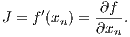
This equation must be solved for xn. The obtained solution must be plugged into f′(xn). The stable range can then be determined.
Abbildung 28: Ducati orbits according to Martynova & Orlov (2009) and rotated Ducati orbits.
Plotting language: GNUPLOT.
Tabelle 9: Konfidenzlevel der Normalverteilung.
Chapter 4
The 3 constants in (A.285) are obtained analytically by solving the system of 3 linear equations,
But how is it possible to integrate up to ∞ numerically? This question must be solved by the reader.
solar masses.
Chapter 5
Abbildung 29: Further Poincaré surfaces of section in the Hénon-Heiles potential with y = 0 and
vy ≥ 0. Top panel: At E = 0.02. We see only periodic and quasiperiodic orbits. Bottom panel: At
E = 0.125. We see a mixture of periodic, quasiperiodic and chaotic orbits. Plotting language: GNUPLOT.
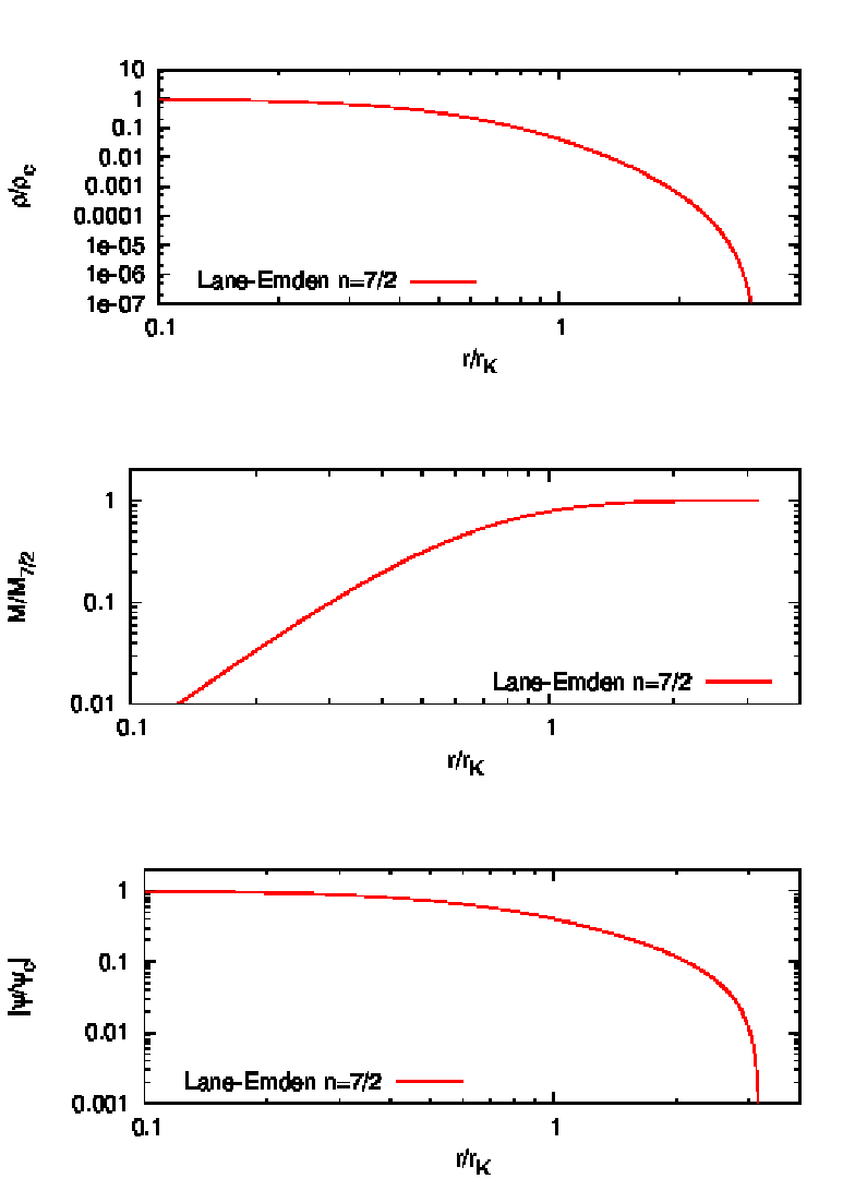
Abbildung 30: Solution of the Lane-Emden equation for a n = 7∕2 polytrope. Top panel: potential.
Middle panel: cumulative mass. Bottom panel: density. Plotting language: GNUPLOT.
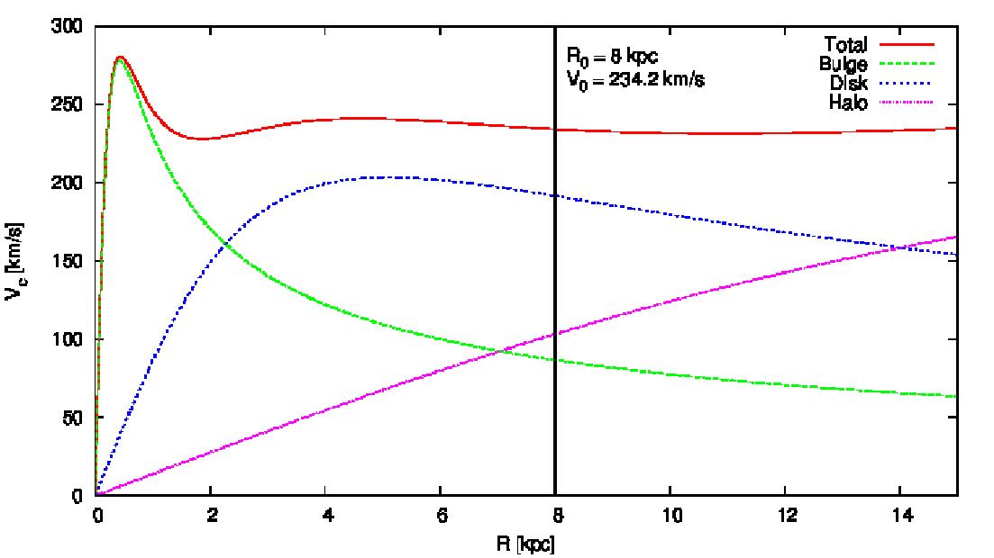
Abbildung 31: Rotation curve of the 3PLK model and its components. The solar radius is marked by
the vertical line at 8 kpc. Plotting language: GNUPLOT.
B TTL program1//-------------------------------------------------------
2// ttl.C 3// Code: Time-transformed leapfrog integrator 4// Ref: S. Mikkola, S. Aarseth, 5// A Time-Transformed Leapfrog Scheme, Cel. Mech. 6// Dyn. Astron., 84 (4), 343-354 (2002) 7// Author: Andreas Ernst 8// Date: Jan 13, 2005 9//------------------------------------------------------- 10 11#include <iostream> 12#include <cmath> 13#include <cstdlib> 14 15using namespace std; 16 17// Calculate accelerations and gradient of Omega function 18 19void acc_and_gradomega(double m[], double r[][3], double a[][3], 20 double grom[][3], int n) { 21 int i, j, k; 22 double (* my_a)[3] = new double[n][3]; 23 double (* my_grado)[3] = new double[n][3]; 24 25 for (i=0; i<n; i++) for (k=0; k<3; k++) { 26 my_a[i][k] = 0; 27 my_grado[i][k] = 0; 28 } 29 30 for (i = 0; i < n; i++) { 31 for (j = i+1; j < n; j++) { 32 double rji[3]; 33 for (k = 0; k < 3; k++) { 34 rji[k] = r[j][k] - r[i][k]; 35 } 36 double r2 = 0; 37 for (int k = 0; k < 3; k++) r2 += rji[k] * rji[k]; 38 double r3 = r2 * sqrt(r2); 39 for (int k = 0; k < 3; k++) { Listing 4: C++ code ttl.C of the time-transformed leapfrog
40 my_a[i][k] += m[j] * rji[k] / r3;
41 my_grado[i][k] += rji[k] / r3; 42 my_a[j][k] -= m[i] * rji[k] / r3; 43 my_grado[j][k] -= rji[k] / r3; 44 } 45 } 46 } 47 48 for (i=0; i<n ; i++) for (k=0; k<3; k++) { 49 a[i][k] = my_a[i][k]; 50 grom[i][k] = my_grado[i][k]; 51 } 52 53 delete my_a; 54 delete my_grado; 55} 56 57// Calculate energy 58 59double energy(double m[], double r[][3], double v[][3], int n) { 60 double ekin = 0, epot = 0; 61 for (int i = 0; i < n; i++) { 62 for (int j = i+1; j < n; j++){ 63 double rji[3]; 64 for (int k = 0; k < 3; k++) rji[k] = r[j][k] - r[i][k]; 65 double r2 = 0; 66 for (int k = 0; k < 3; k++) r2 += rji[k] * rji[k]; 67 epot -= m[i]*m[j]/sqrt(r2); 68 } 69 for (int k = 0; k < 3; k++) 70 ekin += 0.5 * m[i] * v[i][k] * v[i][k]; 71 } 72 return ekin + epot; 73} 74 75// Calculate Omega function 76 77double omega(double m[], double r[][3], int n) { 78 double om = 0; 79 for (int i = 0; i < n; i++) { 80 for (int j = i+1; j < n; j++){ 81 double rji[3]; 82 for (int k = 0; k < 3; k++) rji[k] = r[j][k] - r[i][k]; 83 double r2 = 0; 84 for (int k = 0; k < 3; k++) r2 += rji[k] * rji[k]; 85 om += 1/sqrt(r2); 86 } 87 } 88 return om; 89} Listing 5: C++ code ttl.C of the time-transformed leapfrog
90int main(int argc, char *argv[]) {
91 92// Read initial conditions from stdin, declaration of variables 93 94 int i, j, k; 95 96 if (argc < 3 ) { 97 cout << "Usage:␣ttl␣<dt>␣<t_end>␣<dt_opt>" << endl; 98 return 0; 99 } 100 101 double dt = atof(argv[1]); // time step 102 double t_end = atof(argv[2]); 103 double dt_opt = atof(argv[3]); 104 double t_opt = 0.0; 105 106 int n; 107 cin >> n; 108 109 double t; 110 cin >> t; 111 112 double * m = new double[n]; 113 double (* r)[3] = new double[n][3]; 114 double (* v)[3] = new double[n][3]; 115 double (* a)[3] = new double[n][3]; 116 double (* grado)[3] = new double[n][3]; 117 double (* old_v)[3] = new double[n][3]; 118 119 for (int i = 0; i < n ; i++){ 120 cin >> m[i]; 121 for (int k = 0; k < 3; k++) cin >> r[i][k]; 122 for (int k = 0; k < 3; k++) cin >> v[i][k]; 123 } 124 125// Calculate initial total energy 126 127 double e_in = energy(m, r, v, n); 128 cerr << "Initial␣total␣energy␣E_in␣=␣" << e_in << endl; 129 130 double dt_out = 0.001; 131 double t_out = dt_out; 132 133// Initialize variables 134 135 double W0 = omega(m,r,n); 136 double W = W0, O = 0; 137 t = 0; 138 139// Integration loop Listing 6: C++ code ttl.C of the time-transformed leapfrog
140 while (t < t_end) {
141 142// First step x_{n+1/2} 143 144 for (i=0; i<n; i++) for (k=0; k<3; k++) { 145 r[i][k] += dt*v[i][k]/(2*W); 146 } 147 t += dt/(2*W); 148 149// Second step v_{n+1} 150 151 acc_and_gradomega(m, r, a, grado, n); 152 153 O = omega(m,r,n); 154 155 for (i=0; i<n; i++) for (k=0; k<3; k++) { 156 157 old_v[i][k] = v[i][k]; 158 159 v[i][k] += dt*a[i][k]/O; 160 161 W += dt*(old_v[i][k]+v[i][k])*grado[i][k]/(2*O); 162 } 163 164// Third step r_{n+1} 165 166 for (i=0; i<n; i++) for (k=0; k<3; k++) { 167 r[i][k] += dt*v[i][k]/(2*W); 168 } 169 t += dt/(2*W); 170 171// Data output 172 173 if (t >= t_out) { 174 cout << "DATA:␣"; 175 cout << n << "␣"; 176 cout << t << "␣"; 177 for (int i = 0; i < n; i++) { 178 cout << m[i] << "␣"; 179 for (int k = 0; k < 3; k++) cout << r[i][k] << "␣"; 180 for (int k = 0; k < 3; k++) cout << v[i][k] << "␣"; 181 } 182 cout << endl; 183 t_out += dt_out; 184 } 185// Energy output 186 187 if (t >= t_opt) { 188 double e_cur = energy(m, r, v, n); 189 cerr << "TIME:␣" << t << "␣ENERGY:␣" << e_cur Listing 7: C++ code ttl.C of the time-transformed leapfrog
190 << "␣DEE:␣" << (e_cur - e_in)/e_in << endl;
191 t_opt += dt_opt; 192 } 193 194 } 195 196 double e_out = energy(m, r, v, n); 197 cerr << "Initial␣total␣energy␣E_in␣=␣" << e_in << endl; 198 cerr << "Final␣total␣energy␣E_out␣=␣" << e_out << endl; 199 cerr << "absolute␣energy␣error:␣E_out␣-␣E_in␣=␣" 200 << e_out - e_in << endl; 201 cerr << "relative␣energy␣error:␣(E_out␣-␣E_in)␣/␣E_in␣=␣" 202 << (e_out - e_in) / e_in << endl; 203 204 delete m; 205 delete r; 206 delete v; 207 delete a; 208 delete grado; 209 delete old_v; 210 211 return 0; 212} 213//--------------------------------------------------------- Listing 8: C++ code ttl.C of the time-transformed leapfrog
C Gnuplot examplesPlot data file:
plot "out" u 2:8 lt 1 lw 4 ps 5 w l
replot "out" u 2:10 lt 2 pt 7 ps 5
Plotting styles: Symbol type: pt, symbol color: lt, line width: lw, point size: ps Global point size:
set pointsize 10
set pointsize 0.1
3D Plot:
set view 45,45
splot "out" u 4:5:6
Palette Plot, color bar for 5th column:
set view map
set palette rgbformulae 22,13,-31 splot "out" u 2:4:5 pal
Plot function:
f(x)=x**2
plot [0.0001:1000] f(x) lt 2 pt 7 lw 4
Logarithmic plots:
set logscale x
set logscale y set logscale xy unset logscale x unset logscale y unset logscale xy
Set plot range:
set xrange [-2:2]
set yrange [-2:2]
Plot to Postscript file:
set terminal postscript enhanced color
set output "out.ps" set terminal x11 set output
Axis Labels and Plot Titles:
set xlabel "{/Symbol r}/{/Symbol r}_0"
set ylabel "dE/E_{in}" set title "Kepler problem"
Parametric Plots (e. g. Lissajous figures):
set parametric
plot [0:10*pi] sin(t),cos(t) plot [0:10*pi] sin(t),cos(3*t) plot [0:10*pi] sin(t),cos(4*t) plot [0:10*pi] sin(t),cos(3*t+pi/4)
Plot vertical line with inlined data:
plot "-" w l lt 1 notitle
5 0 5 1 e
Plot different functions in different ranges:
plot (x<=0.08)||(x>=0.5)?1/0:f(x) lt 1 notitle,\
(x<=0.5)||(x>=1.0)?1/0:g(x) lt 2 notitle,\ (x<=1.0)?1/0:h(x) lt 3 notitle
Grid points:
set grid
Label, Arrows:
set label "(0,0) first" at first 0, first 0
set label "(0,0) graph" at graph 0, graph 0 set label "(0,0) screen" at screen 0, screen 0 set arrow from 0,0 to 1,1 set arrow from 0,0 to 1,2 set arrow from 0,0 to 1,3 set noarrow 2 set arrow 3 to 1,5
Fitting with Gnuplot:
f(x) = (1+x**2/a**2)**-2.5
FIT_LIMIT = 1e-10 a = 1.154 fit [0.1:4] f(x) "out3" u 2:4 via a plot f(x) lt 1 title "Plummer a = 1.154 r_0",\ "out3" u 2:4 w l lt 2 title "King W_0=3"
Multiple Plots:
set multiplot
set size square 0.3, 0.5 set origin 0.0, 0.5 set title "V_0 = 0.5 v_{cir}" plot "out11" u 4:5 w l notitle set origin 0.0, 0.0 set title "V_0 = 0.5 v_{cir}" plot "out21" u 4:5 w l notitle ... unset multiplot D Three-body animationsYou need two GNUPLOT scripts, anim.gnu und loop.gnu, with the following commands: anim.gnu:
set nokey
set pointsize 3 set xrange [-3:3] set yrange [-3:3] n=1 c=0.001 load ’loop.gnu’ loop.gnu:
plot ’out’ ev ::n::n u 5:6 pt 7,\
’out’ ev ::n::n u 12:13 pt 7,\ ’out’ ev ::n::n u 19:20 pt 7 print "Step ",n+1 pause c n=n+1; reread The file out is the output generated by the integrator with (x,y) in the (5-th, 6-th), (12-th, 13-th) und (19-th, 20-th) column for the particles 1, 2 und 3.
. | |||||||||||||||||||||||||||||||||||||||||||||||||||||||||||||||||||||||||||||||||||||||||||||||||||||||||||||||||||||||||||||||||||||||||||||||||||||||||||||||||||||||||||||||||||||||||||||||||||||||||||||||||||||||||||||||||||||||||||||||||||||||||||||||||||||||||||||||||||||||||||||||||||||||||||||||||||||||||||||||||||||||||||||||||||||||||||||||||||||||||||||||||||||||||||||||||||||||||||||||||||||||||||||||||||||||||||||||||||||||||||||||||||||||||||||||||||||||||||||||||||||||||||||||||||||||||||||||||||||||||||||||||||||||||||||||||||||||||||||||||||||||||||||||||||||||||||||||||||||||||||||||||||||||||||||||||||||||||||||||||||||||||||||||||||||||||||||||||||||||||||||||||||||||||||||||||||||||||||||||||||||||||||||||||||||||||||||||||||||||||||||||||||||||||||||||||||||||||||||


![∑N xij
ai = - mj x3- (1.43)
j=j⁄=1i ij
N { }
a˙ = -∑ m vij- 3xij(xij ⋅vij) (1.44)
i j=1 j x3ij x5ij
j⁄=i
∑N { a 6v (x ⋅v ) 3x [ 5(x ⋅v )2 ]}
a(2i) = - mj -i3j- --ij--ij5--ij-+ --i5j --ij2-ij--- vij ⋅vij - xij ⋅aij (1.45)
j=1 xij xij xij xij
j⁄=i { [ ]
(3) ∑N ˙aij 9aij(xij ⋅vij) vij 45(xij ⋅vij)2
ai = - mj x3ij - x5ij - x5ij 9vij ⋅vij + 9xij ⋅aij - x2ij
j=j⁄=1i
[
- xij 3xij ⋅a˙ij + 9vij ⋅aij - 45(xij ⋅vij)(xij ⋅aij)
x5ij x2ij
3]}
- 45(xij ⋅vij2)(vij ⋅vij)-+ 105(xij4⋅vij) (1.46)
xij xij](simplyhtml36x.png)
![[( ) ( ) ( )( )]
∑3 ∂X- ∂Y- ∂X- ∂Y-
{X,Y } = ∂xi ∂vi - ∂vi ∂xi
i=1](simplyhtml38x.png)

 is the time evolution “operator”. The time evolution of each component of

 is called the “Hamiltonian flow”.
![1 3 3 2 2
Z ≈ X + Y + 2[X, Y]+ O (X ,Y ,X Y,XY )](simplyhtml47x.png)


 .
A typical non-commutative operation from every-day life is, for example, washing and drying
clothes.
.
A typical non-commutative operation from every-day life is, for example, washing and drying
clothes.
![Γ = ϵ[log(T - P )- log(V)].
0](simplyhtml65x.png)


 be a scheme of order
 is the Wick-Dyson time ordering
operator. We refer to
is the Wick-Dyson time ordering
operator. We refer to 


![3 ∫ ∞ ∞ ∫ ∞ d [ ] W
Π = 2 ⋅4π ρ(r)σ2(r)r2dr = 2πr3ρ(r)σ2(r)|0-- 2π dr ρ(r)σ2(r) r3dr = C --2-,
0 ◟ ◝C◜ ◞ 0](simplyhtml125x.png)


![[ ( )2-γ]
Φ(r) = - GM--1--- 1- -r---
a 2- γ r+ a](simplyhtml138x.png)

![( ) ( ) ( x )
( ax ) (dΦ ∕dx) ----------- GM------------ ( y )
ay = - dΦ∕dy = [2 2 √ 2---2-2]3∕2 ⋅ a+√b2+z2
az dΦ∕dz x + y + (a+ b + z) z ⋅ √b2+z2](simplyhtml148x.png)
![{ [ ( ) ] [ ( √------)2]}
dax GM---3x--xvx +-yvy +-zvz-√b2a+z2-+1----vx-x2 +-y2 +-a-+-b2 +-z2---
dt = [ ( √------)2]5∕2
x2 + y2 + a + b2 + z2](simplyhtml149x.png)
![{ [ ( )] [ ( √ ------) ]}
da GM 3y xvx + yvy + zvz √-2a-2-+1 - vy x2 + y2 + a + b2 + z2 2
--y = -------------------[-----b+z(----√------)-]5∕2-------------------
dt x2 + y2 + a + b2 + z2 2](simplyhtml150x.png)
![{
daz a+ √b2-+-z2[ ( a ) ]
dt-= GM 3z--√-2---2-- xvx + yvy + zvz √-2---2-+1
[ b + z ] [ ( b√-+-z--) ]}
2 2 ( ∘ -2---2)2 -a+--b2-+z2-- 2----a-----
- vz x + y + a+ b + z × √b2-+-z2 - z (b2 +z2)3∕2 /
[ ]5∕2
x2 + y2 + (a +∘b2-+-z2)2 (2.171)](simplyhtml151x.png)


![( ) ( ) [ ] ( )
¨x = - ∂Φ ∕∂x = - x2 (1 + 2y) = 0
¨y - ∂Φ ∕∂y - x - y(1- y) 0](simplyhtml182x.png)


 , where


![[1 - n - n ]
Jmn = λn 2λ(n -11)
2 1](simplyhtml198x.png)
![2
det(J - λ1) = λ - λ[λ(n1 - 1)- (n2 - 1)]+λ (n1 + n2 - 1) = 0](simplyhtml199x.png)
![∘ ------------------2---------------
λ1,2 = - 1[λ(n1 - 1)- (n2 - 1)]± [λ-(n1---1)--(n2---1)]-- λ(n1 + n2 - 1)
2 4](simplyhtml200x.png)
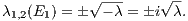
![[λ1,2(E1)]](simplyhtml202x.png)

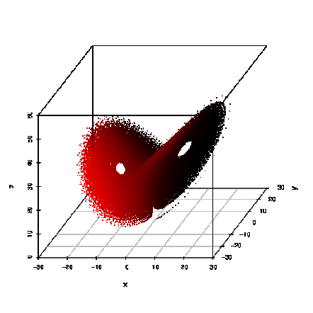
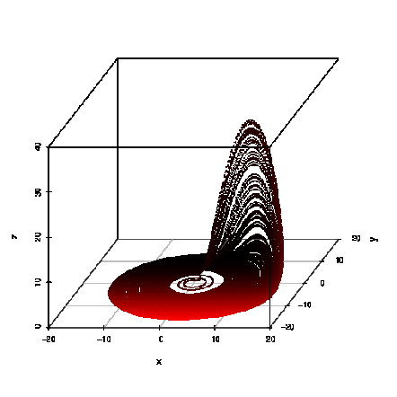
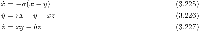


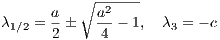
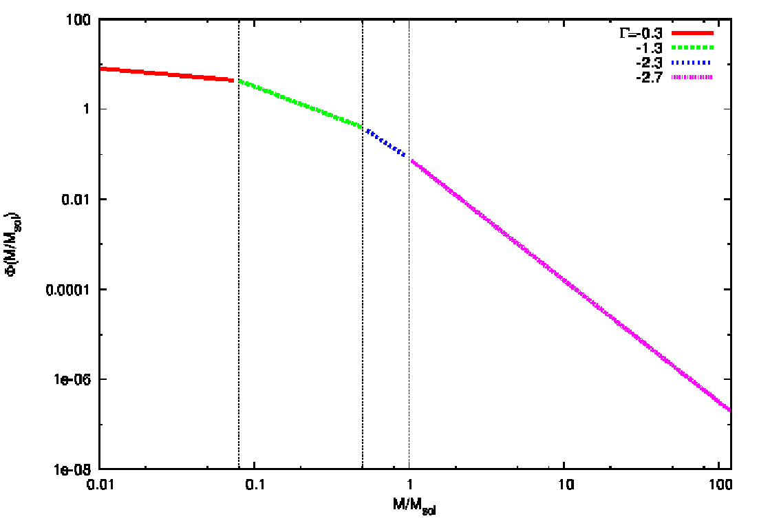


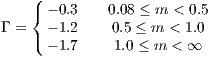

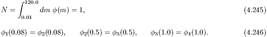

![120.0∕h
∑ h-
N ≈ [ϕ(m) +ϕ (m + h)]× 2
0.01∕h](simplyhtml225x.png)
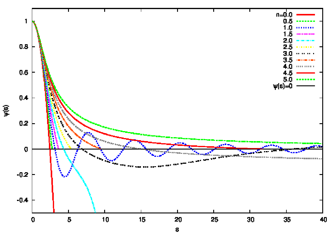


![[ Φ ]n
ρ = - (n-+1)K-](simplyhtml229x.png)
![( ) [ ]
-1-d 2dΦ- ----Φ--- n
r2dr r dr = 4πG -(n + 1)K .](simplyhtml230x.png)
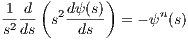
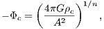
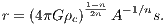

![[ ]-n-
ρ = --4πG--- 1-n ( r)12n-n .
c (n+ 1)K s](simplyhtml237x.png)
![∫
M = 4π R r2ρdr (5.263)
0
3-23nn -3∕n ∫ s1 2 n
= 4π(4πG ρc) A ρc 0 s ψ (s)ds (5.264)
3-n 3∕2∫ s1 ( )
= - 4π ρ2cn-(4πG)3-23nn[(n+-1)K]-- d- s2dψ- ds (5.265)
(4πG)3∕(2n) 0 ds ds
3-n-[(n+ 1)K ]3∕2[ dψ]
= - 4π ρ2cn -------- s2--- . (5.266)
4πG ◟--d◝s◜-s1◞
-Mn](simplyhtml238x.png)
![[s2dψ∕ds]](simplyhtml239x.png)
![( )n-1( )3-n n
GM-- -R- = [(n-+-1)K-]-
Mn Rn 4πG](simplyhtml240x.png)
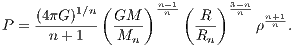
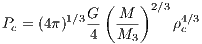

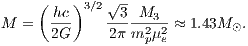
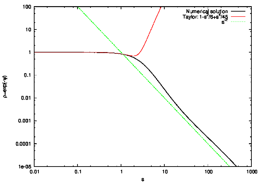
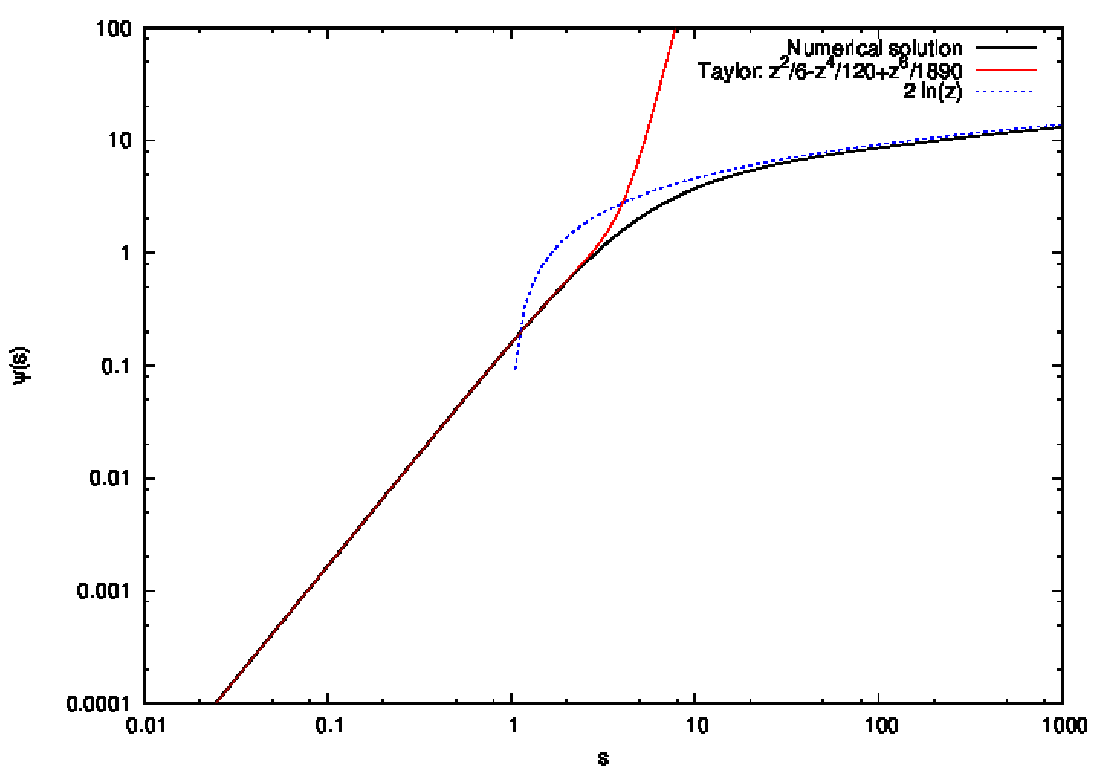
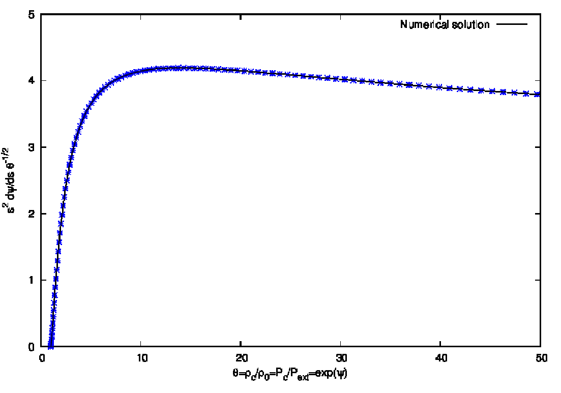
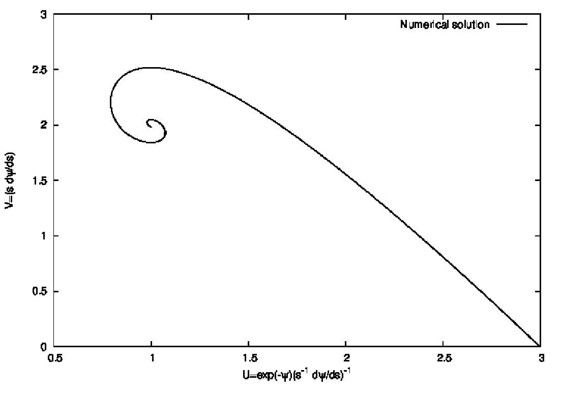
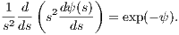
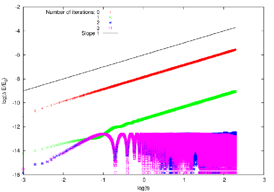


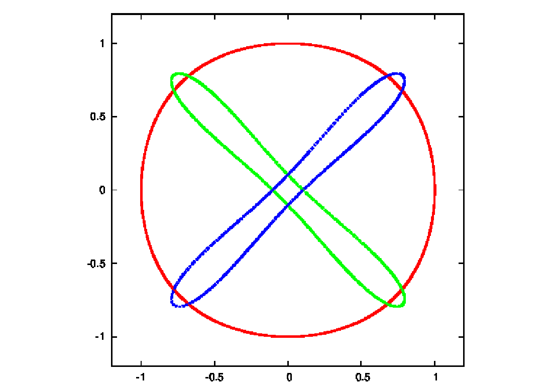
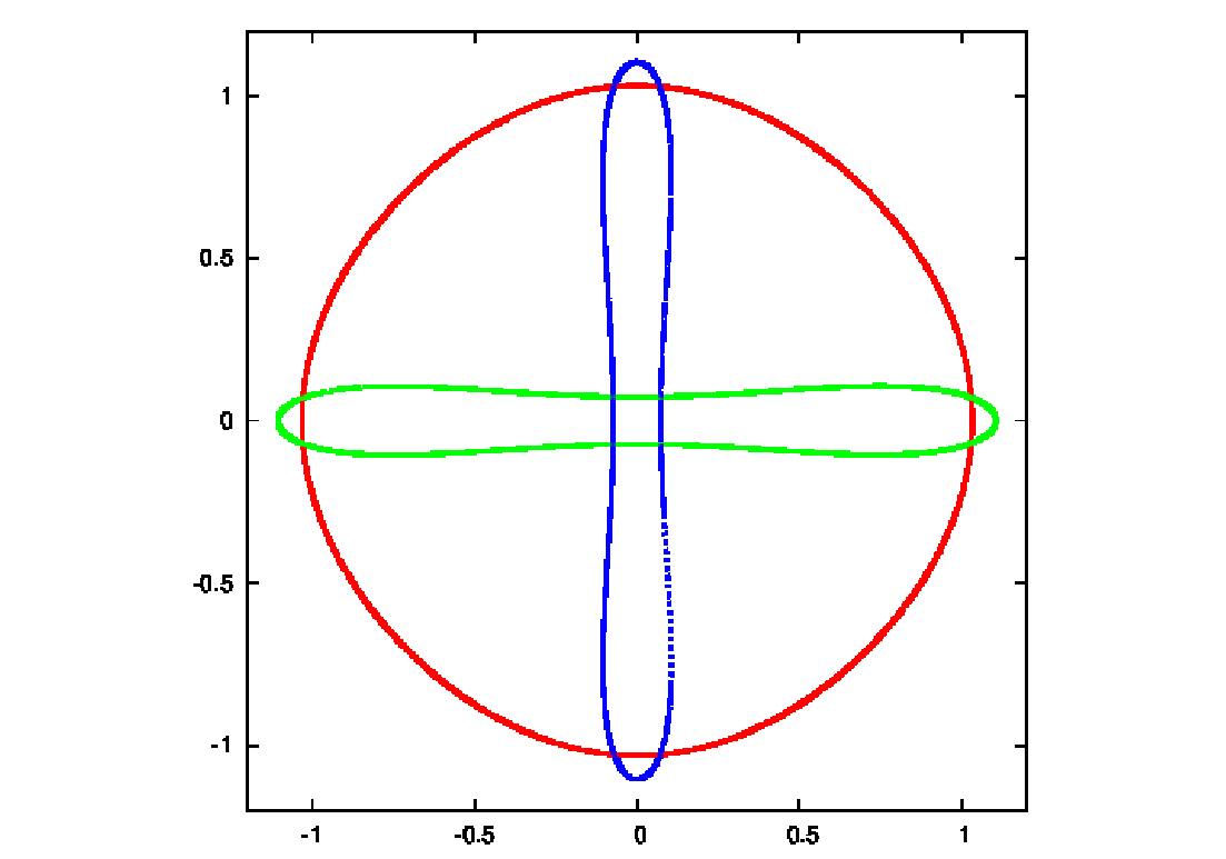
![[ 2 2]
- x ∕(2σ )](simplyhtml259x.png)

![[ 2 2 ]
- x∕(2σ )](simplyhtml261x.png)

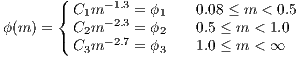


 and units
where used in which
and units
where used in which